last revision: December 1, 2019
This is the syntax which was used to process the raw data file from the Commodity Futures Trading Commission (CFTC) through to the final results published in:
Posch, Konrad, Nath, Thomas and Ziegler, J. Nicholas. “The Limits of Interest: Capture, Financialization, or Contestation in the Politics of Rule-Making for Derivatives”
Narrative online Appendices: (Posch, Nath, & Ziegler 2019-11-24) The Limits of Interest – Watson Working Paper – Online Appendices
Syntax appear below:
- Setup Environment
- 0. Prepare Corpus
- 1. Estimate Mallet Topics
- 2. Substantive Analyses of Groups of Comments (sub-Corpora)
- 3. Who Commented on the 10 most commented rules in the Coded (8k) dataset
- 4. Deprecated Additional Analyses
While the dataset was produced from internal CFTC servers (because the CFTC did not participate in Regulations.gov in 2014), they explicitly only provided publicly available data. Thus, the full dataset of 37,703 comments will be available from Dryad (https://doi.org/10.6078/D1610G) upon publication along with the codebook provided by the CFTC and amended with our additional classification variables as used below and described in the manuscript and online supporting information C.
It should be noted that the CFTC does have additional meta-data which they declined to provide (i.e. IP addresses for commenters and other personally identifiable information) which they noted could be obtained through a Freedom of Information Act (FOIA) request. We did not pursue this avenue, but future researchers interested in, for example, the geographic distribution of commenters could request such data.
The Latent Dirichlet Analysis (LDA) used here is executed with Mallet. Mallet is a popular topic modelling software application. Mallet is written in java – which means it’s fast – and R has a Mallet wrapper package – which means it’s more userfriendly.
However, Mallet is a very resource-heavy app (because Java loves to use resources) so optimizing the number of working threads is key to running the code in a reasonable amount of time. Details are provided in the Setup Environment syntax, but the gist is you want to experiment with the number of threads based on your configuration to get the fastest runtime possible. Runtime for the 12,000 iteration topic model used to generate results for publication took on the order of 36 minutes using a Ryzen 3600 CPU (6 core, 12 logical processors, 4.1Ghz, 12 threads). The old Phenom II 720 processor (3 core, 3 logical processors, 3.5GHz, 15 threads) took on the order of 3.5 hours. Configuration and processor power matter a great deal to how this code runs (although anything can run it eventually).
NOTE: While it should NOT affect the stability of results, apparently the number of threads does. There is an element of randomness to topic modelling so while topics created from a corpus run with different random seeds will be substantively similar, they may appear in different orders and with slightly different topic proportions. To create reproducible results, this syntax sets the random seed (see section 1.2.1). However, it also appears that the number of threads is affecting output as well, so if you would like to exactly reproduce our results in the manuscript, you need to leave the “number of logical processors” value (numLogicalProcessors) in Section 0 set to 15.
Setup Environment
##clears R memory
rm(list=ls())

## Mallet is a massive pig when it comes to processing (roughly 11 seconds/10 iterations).  Enter the number of logical processors below to enable multi-threading
numLogicalProcessors = 15

# Set the number of iterations. 1000 for testing, 12000 for analysis
iterations <- 12000


## desktop wd
wd <- "D:/Dropbox/The Limits of Interest"

## Laptop wd
#wd <- "C:/Dropbox/The Limits of Interest"

setwd(wd)


## install REQUIRED non-default packages if not yet installed
#install.packages(c("mallet","rJava","RTextTools","SnowballC","plyr","dplyr","ggplot2","reshape2","xtable","qdap","knitr","viridis"))

#######################################################################################
##                                                                                   ##
##  NOTE: For mallet to work, you must install the Java Development Kit (JDK)        ##
##       not just the runtime environment (JRE).  This is free on the java website,  ##
##       but must be installed on your system before you can call the mallet         ##
##       library below.                                                              ##
##                                                                                   ##
#######################################################################################


options(java.parameters = "-Xmx8000m") #this is the magic solution to the out of memory error as Mallet limits RAM usage to 1gb which is much too small for our dataset

# load REQUIRED libraries
library(rJava) # the interface between R and Java, needed for mallet
library(mallet) # a wrapper around the Java machine learning tool MALLET
library(SnowballC) # for stemming
library(tm) # Framework for text mining
#library(RTextTools) # a machine learning package for text classification written in R
library(plyr)
library(dplyr) # Data preparation and pipes $>$
library(ggplot2) # for plotting word frequencies
library(scales)
library(stringr)
library(reshape2) #visualization
library(xtable) # pretty tables
library(knitr) # final output and file handling
library(viridis) #Inclusive design palettes for stacked bar charts because inclusive design is good design
0. Prepare Corpus
This module reads in the raw data and prepares it for topic modeling.
0.0 Combine the CFTC raw data file with the organization codings in this file from (2017-05-11) syntax file
The CFTC provided all comments submitted during the public comment periods on all rules they have written to implement the Dodd-Frank Act.
It is INCREDIBLY important that this combination happen in R and not Excel as Excel has a 32,765 (32,767-2 text qualifier “) character limit for it’s cells and it will truncate any data placed in there. There are a number of comment letters which are longer than this limit (ex. 8895, 26166, 26171) so all matching and processing MUST happen in R.
Note: the original data file had to be changed to UTF-8 from unknown (possibly Unicode) format using Notepad.exe because otherwise nothing showed up in R.
# load data
cftc.Comments <- read.delim("D:/Dropbox/The Limits of Interest/DoddFrankCommentsAll(UTF-8).txt",
                            sep="|",
                            header=TRUE,
                            stringsAsFactors = FALSE,
                            encoding ="UTF-8",
                            strip.white = TRUE,
                            quote = "" #this is a unbelieveably vital inclusion otherwise you lose cases!
                            ) ##These are the comments on proposed regulations (NPRMs)

####Check to see if we have unexpected blank data on import, esp. in CommentText
sum(1*(cftc.Comments$CommentText=="")) # 1036 Expected, although will be only 86 for cases we analyze, see 0.1 below
## [1] 1036#CHeck the variable names
names(cftc.Comments)## [1] "X.U.FEFF.ControlNumberID" "SubmitDate"
## [3] "UniqueName" "FirstName"
## [5] "LastName" "Organization"
## [7] "Title" "CommentText"
## [9] "ExtractedText"#Fix the oddly named first variable
colnames(cftc.Comments)[1] <- "ControlNumberID"
names(cftc.Comments)## [1] "ControlNumberID" "SubmitDate" "UniqueName" "FirstName"
## [5] "LastName" "Organization" "Title" "CommentText"
## [9] "ExtractedText"#load in the classified Organization values and meta-data
cftc.Comments.metaData<-read.csv("D:/Dropbox/The Limits of Interest/(2019-06-12) Final Classifications for R_noText.csv", stringsAsFactors = FALSE)
####################################################################
#CHeck the variable names
names(cftc.Comments.metaData)## [1] "ControlNumberID"
## [2] "SubmitDate"
## [3] "UniqueName"
## [4] "FirstName"
## [5] "LastName"
## [6] "Organization"
## [7] "Title"
## [8] "In.NZ.and.LE.memos"
## [9] "Rule.Super.set..from.Memo.Title."
## [10] "Vlookup.Key"
## [11] "Final.Classification"
## [12] "Final.Classification.Multivalue.2"
## [13] "Final.Classification.Multivalue.3"
## [14] "Final.Classification.Multivalue.4"
## [15] "Final.Classification.Multivalue.5"
## [16] "VA.KSC.Classification"
## [17] "VA.KSC.Multivalue.2"
## [18] "VA.KSC.Multivalue.3"
## [19] "VA.KSC.Multivalue.4"
## [20] "VA.KSC.Multivalue.5"
## [21] "VA.KSC.Non.US...Non.US.or.Blank."
## [22] "LE.Classification"
## [23] "LE.Multivalue.2"
## [24] "LE.Multivalue.3"
## [25] "LE.Multivalue.4"
## [26] "LE.Non.US...Non.US.or.Blank."#Fix the oddly named first variable
colnames(cftc.Comments.metaData)[1] <- "ControlNumberID"
names(cftc.Comments.metaData)## [1] "ControlNumberID"
## [2] "SubmitDate"
## [3] "UniqueName"
## [4] "FirstName"
## [5] "LastName"
## [6] "Organization"
## [7] "Title"
## [8] "In.NZ.and.LE.memos"
## [9] "Rule.Super.set..from.Memo.Title."
## [10] "Vlookup.Key"
## [11] "Final.Classification"
## [12] "Final.Classification.Multivalue.2"
## [13] "Final.Classification.Multivalue.3"
## [14] "Final.Classification.Multivalue.4"
## [15] "Final.Classification.Multivalue.5"
## [16] "VA.KSC.Classification"
## [17] "VA.KSC.Multivalue.2"
## [18] "VA.KSC.Multivalue.3"
## [19] "VA.KSC.Multivalue.4"
## [20] "VA.KSC.Multivalue.5"
## [21] "VA.KSC.Non.US...Non.US.or.Blank."
## [22] "LE.Classification"
## [23] "LE.Multivalue.2"
## [24] "LE.Multivalue.3"
## [25] "LE.Multivalue.4"
## [26] "LE.Non.US...Non.US.or.Blank."#check the classifications for Final.Classification
unique(cftc.Comments.metaData$Final.Classification)## [1] "Un-Coded"
## [2] "Private Asset Manager"
## [3] "Market Infrastructure Firm"
## [4] "Law Firms, Consultants, and Related Advisors"
## [5] "Unaffiliated Individual"
## [6] "Non-Financial Firm"
## [7] "Academic or Other Expert"
## [8] "Non-Financial Private-Sector Association"
## [9] "Government"
## [10] "Financial Sector Association"
## [11] "Consumer Advocacy or other Citizens Group"
## [12] "Core Financial Service Trade Association"
## [13] "U.S. Chamber of Commerce or Affiliate"
## [14] "Major Wall Street Sell-Side Bank"
## [15] "Public Asset Manager"
## [16] "Other Sell-Side Bank"
## [17] "Trade Union or other Formal Labor Organization"
## [18] "Market Advocacy or other Anti-Regulation Group"Now there are only some of the comments with an organization val, 8568 to be precise. This chunk produces 9450 comments but that includes NA values which are seen as non-empty. Final cull to 8568 happens when matched to Final.Classification
For our analysis, those are the only comments we need to topic model, so let’s cut the database down to size.
# Let's subset out the comments with organization values which are the ones we want
cftc.Comments.withOrg <- subset(cftc.Comments, Organization!="")

# lets count the total number of unique org values
length(unique(cftc.Comments.withOrg$Organization))
## [1] 4752# lets see a few of those
head(unique(cftc.Comments.withOrg$Organization),20)## [1] "NOYB" "Home Communications"
## [3] "khterFX DBA" "FXP Intl"
## [5] "Gain Capital/Forex" "STG Holdings LC"
## [7] "Very" "FX Bridge Technologies"
## [9] "Black Bay FX Services LLC" "Forex Power Net"
## [11] "Forex Trader" "Bay View Trading Corporation"
## [13] "Back Bay FX Services LLC" "ProAct Traders LLC"
## [15] "Forex Community" "Silicon Valley Forex"
## [17] "Partick Smith Realty" "Gami/Tati"
## [19] "Yoder & Associates Inc" "Kelly Industries"# see a truncated version of this now smaller data, truncdf seems to be deprecated after R 2.3.2
#head(truncdf(cftc.Comments.withOrg,10))Finally, we need to load in the meta-data related to classification and super group
#First, drop the duplicate metadata
cftc.Comments.metaData <- subset(cftc.Comments.metaData, select=c(
ControlNumberID
,In.NZ.and.LE.memos
,Rule.Super.set..from.Memo.Title.
,Final.Classification
,Final.Classification.Multivalue.2
,Final.Classification.Multivalue.3
,Final.Classification.Multivalue.4
,Final.Classification.Multivalue.5
,VA.KSC.Classification
,VA.KSC.Multivalue.2
,VA.KSC.Multivalue.3
,VA.KSC.Multivalue.4
,VA.KSC.Multivalue.5
,VA.KSC.Non.US...Non.US.or.Blank.
,LE.Non.US...Non.US.or.Blank.
,LE.Classification
,LE.Multivalue.2
,LE.Multivalue.3
,LE.Multivalue.4)
)

#merge the meta-data dataframe with the comment dataframe, NOTEL this drops 889 cases (9457->8568 which are some version of none or N/A as entered in the original dataset by the commenter)
cftc.Comments.withOrgAndMeta<- merge(cftc.Comments.withOrg, cftc.Comments.metaData, by="ControlNumberID")

#Lets see where we have some missing data in text variables (such as ExtractedText)
sum(1*(cftc.Comments.withOrgAndMeta$ExtractedText=="")) #should be 5, some of the original file had no text here
## [1] 5sum(1*(cftc.Comments.withOrgAndMeta$CommentText=="")) #should be 86## [1] 86sum(1*(cftc.Comments.withOrgAndMeta$Final.Classification=="")) #should be 0## [1] 0#Reorder the columns so the massive and messy variables of CommentText and Extracted Text appear at the end of the file for cleanliness
names(cftc.Comments.withOrgAndMeta)## [1] "ControlNumberID"
## [2] "SubmitDate"
## [3] "UniqueName"
## [4] "FirstName"
## [5] "LastName"
## [6] "Organization"
## [7] "Title"
## [8] "CommentText"
## [9] "ExtractedText"
## [10] "In.NZ.and.LE.memos"
## [11] "Rule.Super.set..from.Memo.Title."
## [12] "Final.Classification"
## [13] "Final.Classification.Multivalue.2"
## [14] "Final.Classification.Multivalue.3"
## [15] "Final.Classification.Multivalue.4"
## [16] "Final.Classification.Multivalue.5"
## [17] "VA.KSC.Classification"
## [18] "VA.KSC.Multivalue.2"
## [19] "VA.KSC.Multivalue.3"
## [20] "VA.KSC.Multivalue.4"
## [21] "VA.KSC.Multivalue.5"
## [22] "VA.KSC.Non.US...Non.US.or.Blank."
## [23] "LE.Non.US...Non.US.or.Blank."
## [24] "LE.Classification"
## [25] "LE.Multivalue.2"
## [26] "LE.Multivalue.3"
## [27] "LE.Multivalue.4"cftc.Comments.withOrgAndMeta<-cftc.Comments.withOrgAndMeta[c(1:7,10:24,8,9)]
## Write this prepared corpus to a data file
write.table(cftc.Comments.withOrgAndMeta,file="DoddFrankCommentsWithOrgValueAndMetaData.txt",sep="|",row.names = FALSE,quote=FALSE)0.1 Load the Data
First let’s read in our data. The corpus we’ll be using today is a database of CFTC comments related to Dodd-Frank Financial Reform Implementation which was created as described in step 0.0 above.
#read in text, | delimited file
documents <- read.delim("DoddFrankCommentsWithOrgValueAndMetaData.txt",
                            sep="|",
                            header=TRUE,
                            stringsAsFactors = FALSE,
                            quote = "" #this is a unbelieveably vital inclusion otherwise you                                                        lose cases!  This turns off quotes which is important for the full text                                        otherwise cases get wrapped into previous cases.  It is causing all the                                        data read in to have quotes wrapped around it and to have blank values                                        stored as ""
                            ) ##These are the comments on proposed rulemaking

# examine the variables names in our dataset
names(documents)
## [1] "ControlNumberID"
## [2] "SubmitDate"
## [3] "UniqueName"
## [4] "FirstName"
## [5] "LastName"
## [6] "Organization"
## [7] "Title"
## [8] "In.NZ.and.LE.memos"
## [9] "Rule.Super.set..from.Memo.Title."
## [10] "Final.Classification"
## [11] "Final.Classification.Multivalue.2"
## [12] "Final.Classification.Multivalue.3"
## [13] "Final.Classification.Multivalue.4"
## [14] "Final.Classification.Multivalue.5"
## [15] "VA.KSC.Classification"
## [16] "VA.KSC.Multivalue.2"
## [17] "VA.KSC.Multivalue.3"
## [18] "VA.KSC.Multivalue.4"
## [19] "VA.KSC.Multivalue.5"
## [20] "VA.KSC.Non.US...Non.US.or.Blank."
## [21] "LE.Non.US...Non.US.or.Blank."
## [22] "LE.Classification"
## [23] "CommentText"
## [24] "ExtractedText"#Lets see where we have some missing data in text variables (such as ExtractedText)
sum(1*(documents$ExtractedText=="")) #should be 5## [1] 5sum(1*(documents$CommentText=="")) #should be 86## [1] 86#confirm that every comment has a classification
sum(1*(documents$Final.Classification=="")) #should be 0## [1] 00.1.1 Drop Ex Parte Meetings and Comments “None” type values in Organization
The CFTC included 286 ex parte meetings in their dataset. Since the data generating process for those comments is not the same as that for the other comments, we need to drop them from the analysis. These cases can be identified based on the value "Ex Parte" in the FirstName variable.
There are also 20 cases with organization values which are uninterpretable. They must be dropped
#Check the number of ex parte meetings
sum(1*(documents$FirstName=="Ex Parte")) #should be 286
## [1] 286# Subset the data to include only those cases which are not ex parte meetings
documents <- subset(documents, FirstName!="Ex Parte")
# verify that the correct number of comments remain
nrow(documents) #should be 8282## [1] 8282# create the list of junk org values
junkOrgValues <- c("(NONE)",".","/","[none]","-none-","None","None ","None.","none","none ","none.")
junkOrgValues## [1] "(NONE)" "." "/" "[none]" "-none-" "None" "None "
## [8] "None." "none" "none " "none."#check number of comments with junk org values
sum(1*(documents$Organization %in% junkOrgValues)) #should be 20## [1] 20# Subset the data to include only those cases which do not have junk organization values
documents <- subset(documents, !(Organization %in% junkOrgValues))
# verify that the correct number of comments remain
nrow(documents) #should be 8262## [1] 82620.1.2 Get Unique Organization Values from the Corpus for Data Coding Purposes
In order to code comments to our typology, we need a list of all unique values in the Organization variable.
# count the number of unique values in Organization
length(unique(documents$Organization)) #should be 4671
## [1] 4603# get the unique list of Organization values with counts of relevant comments
validOrgValues <- as.data.frame(table(documents$Organization))
colnames(validOrgValues)[1]<- "Organization"
## look at the first 30 and notice that we have a number that are conceptually identical but technically distinct due to trival variations such as punctuation and spacing. These are solved by conceptual coding to avoid accidental loss of data
head(validOrgValues, 30)## Organization
## 1 - National Rural Electric Cooperative Association;®- American Public Power Association; and®- Large Public Power Council.
## 2 (a private individual)
## 3 (individual)
## 4 (none; private investor, retired from career in banking and finance)
## 5 (Private Investor)
## 6 ® ®Eden Earth Resources LLC
## 7 ®Free citizen, tax payer, and in 10 years been promised a social security payback
## 8 ®self
## 9 00
## 10 1,500 contracts is a fair and appropriate position limit in silver. 1,500 should be the maximum (or 7 million ounces). The proposed limit of 5,000 + will not solve the manipulation problem in silver.
## 11 17 CFR (SDR)®79 FR 16672
## 12 19 Community and Regional Banks
## 13 1st Infantry Division, Combat Aviation Brigade
## 14 25th Aviation
## 15 36 South
## 16 3Degrees Group, Inc.
## 17 3F Forecasts
## 18 401K owner
## 19 56 National coalitions and organizations and ®28 International coalitions and organizations from 16 countries
## 20 56 National coalitions and organizations and®28 International coalitions and organizations from 16 countries
## 21 79 FR 1347 (17 CFR)
## 22 965
## 23 A Bonvouloir
## 24 A citizen for a fair and just society.
## 25 a concerned citizen of united states of America
## 26 A dad!!!
## 27 A regional bank
## 28 A screwed American due to the Corruption that is so widespread throughout the Government including the CFTC.
## 29 A slave to the corrupt system.
## 30 A Slave to the system.
## Freq
## 1 1
## 2 1
## 3 1
## 4 1
## 5 1
## 6 1
## 7 1
## 8 1
## 9 1
## 10 1
## 11 1
## 12 2
## 13 1
## 14 1
## 15 1
## 16 1
## 17 1
## 18 1
## 19 1
## 20 1
## 21 1
## 22 1
## 23 2
## 24 1
## 25 1
## 26 1
## 27 3
## 28 1
## 29 1
## 30 1## Sort in decending order of frequency to see top values
validOrgValues <- validOrgValues[order(validOrgValues$Freq, decreasing = TRUE),]
## examine the top 30 most common raw values, notice seemingly identical values which are actually slightly different necessitating manual conceptual coding by analysts
head(validOrgValues, 30)## Organization
## 3702 self
## 3703 Self
## 251 Americans for Financial Reform
## 3306 Private Investor
## 1848 Individual
## 477 Better Markets, Inc.
## 1982 Investor
## 2416 Managed Funds Association
## 1861 Individual Investor
## 3303 private investor
## 3305 Private investor
## 1847 individual
## 3259 private citizen
## 3261 Private Citizen
## 3466 Retired
## 3253 Private
## 3252 private
## 845 Coalition of Physical Energy Companies (COPE)
## 1752 Hunton & Williams LLP
## 3260 Private citizen
## 506 BlackRock, Inc.
## 1387 Financial Services Roundtable
## 2451 MarkitSERV
## 777 Citizen
## 1860 Individual investor
## 4338 United States Senate
## 2009 ISDA
## 3465 retired
## 344 Asset Management Group, Securities Industry and Financial Markets Association
## 4090 The Depository Trust & Clearing Corporation
## Freq
## 3702 91
## 3703 79
## 251 76
## 3306 76
## 1848 73
## 477 60
## 1982 59
## 2416 55
## 1861 50
## 3303 50
## 3305 47
## 1847 44
## 3259 44
## 3261 39
## 3466 38
## 3253 36
## 3252 35
## 845 33
## 1752 33
## 3260 33
## 506 30
## 1387 30
## 2451 30
## 777 29
## 1860 29
## 4338 29
## 2009 28
## 3465 28
## 344 26
## 4090 26## For easy coding, sort validOrgValues alphabetically by Organization column
validOrgValues <- validOrgValues[order(validOrgValues$Organization, decreasing = FALSE),]
## Write that list to a | delimited file for easy copy into excel and sending to coders
filename = paste("Unique_Valid_Organization_Values_withCounts_",nrow(documents),"_comments_",format(Sys.time(), "%Y-%m-%d_%H.%M.%S"),".txt", sep="")
write.table(validOrgValues, row.names=FALSE, col.names=TRUE, file = filename, sep = "|")
filename## [1] "Unique_Valid_Organization_Values_withCounts_8262_comments_2019-12-01_11.57.15.txt"0.2 Created a unified text column to solve the gaps in CommentText and ExtractedText
As seen above in section 0.1, there are 5 blank values in ExtractedText. We need to create a unified text column called UnifiedText which includes a value for all comments by filling the 5 blanks with the values from CommentText.
## View the 5 comments which have missing ExtractedText values and confirm that they have CommentText Values
#   Truncate the printout so we don't get a mess

str_trunc(documents[documents$ExtractedText=="",]$CommentText,300) #only 5 results expected, confirm that all [index] numbers are followed by non-NULL values that look like comment letter text
## [1] "Dear Sirs:®®There has been way too much interference with the silver market by certain big players, artificially keeping prices totally out of realistic market ranges. The CFTC and the Comex were never designed to facilitate market manipulation, but with the existing rules, that has become the c..."
## [2] "Futures are used in the real world to control costs, protect profits, reduce liability. Real people, producing real commodities, producing real good that people use and consume.®Of they are also used as a trading vehicle, of which I consider some trading to be useful as to a price discovery.®®B..."
## [3] "You must not allow more than 1,500 contracts as the appropriate concentration limit for the COMEX Silver market. Our liberty is directly related to this issue."
## [4] "I urge you to please curb excessive gambling in commodities markets like food and oil. ®®While many factors contribute to today’s highly volatile commodity prices, it is clear that excessive speculation is significantly responsible, as shown in dozens of studies by several respected institutions ..."
## [5] "Title: End-User Exception to Mandatory Clearing of Swaps®FR Document Number: 2010-31578®Legacy Document ID: ®RIN: 3038-AD10®Publish Date: 12/23/2010 12:00:00 AM®®Submitter Info:®First Name: Fred®Last Name: Nadelman, LMSW®Mailing Address: 1825 East Gwinnett Street®City: Savannah®Country: Unit..."## Create a new combined text variable which will be used for anlysis called "UnifiedText" and populate it with ExtractedText for all 8257 comments (total comments minus 5) which have a value for ExtractedText.
documents$UnifiedText <- documents$ExtractedText
## Fill the 5 missing values in ExtractedText using CommentText and save to new variable UnifiedText
documents[documents$ExtractedText=="",]$UnifiedText <- documents[documents$ExtractedText=="",]$CommentText
## Confirm that UnifiedText has no empty values
sum(1*(documents$UnifiedText=="")) #should be 0## [1] 0## Confirm that the 5 comments which had missing ExtractedText values have CommentText values in UnifiedText
documents[documents$ExtractedText=="",]$UnifiedText == documents[documents$ExtractedText=="",]$CommentText #should be 5 TRUE values## [1] TRUE TRUE TRUE TRUE TRUE0.3 Make the 18-part typology a factor
Now, for representativeness, we need to convert the 18 part typology (17 substantive categories + 1 “Un-coded”) into a factor because the typology was constructed to span a spectrum roughly from industry insider (top) to general public (bottom) with the residual category of “Un-Coded” at the end.
## confirm that Final.Classification has no erroneous spellings (should have 18 unique values)
unique(documents$Final.Classification)
## [1] "Un-Coded"
## [2] "Private Asset Manager"
## [3] "Market Infrastructure Firm"
## [4] "Law Firms, Consultants, and Related Advisors"
## [5] "Unaffiliated Individual"
## [6] "Non-Financial Firm"
## [7] "Academic or Other Expert"
## [8] "Non-Financial Private-Sector Association"
## [9] "Government"
## [10] "Financial Sector Association"
## [11] "Consumer Advocacy or other Citizens Group"
## [12] "Core Financial Service Trade Association"
## [13] "U.S. Chamber of Commerce or Affiliate"
## [14] "Major Wall Street Sell-Side Bank"
## [15] "Public Asset Manager"
## [16] "Other Sell-Side Bank"
## [17] "Trade Union or other Formal Labor Organization"
## [18] "Market Advocacy or other Anti-Regulation Group"##c creates a vector of the different typologies
documents$Final.Classification <- factor(documents$Final.Classification, levels = c(
"Major Wall Street Sell-Side Bank",
"Other Sell-Side Bank",
"Core Financial Service Trade Association",
"Financial Sector Association",
"Public Asset Manager",
"Private Asset Manager",
"U.S. Chamber of Commerce or Affiliate",
"Market Infrastructure Firm",
"Law Firms, Consultants, and Related Advisors",
"Non-Financial Private-Sector Association",
"Non-Financial Firm",
"Government",
"Academic or Other Expert",
"Consumer Advocacy or other Citizens Group",
"Trade Union or other Formal Labor Organization",
"Market Advocacy or other Anti-Regulation Group",
"Unaffiliated Individual",
"Un-Coded")
)
# now, verify that we indeed have an ORDERED 17 level typology as listed above (look at [indecies] and confirm it goes in the order listed in the above creation statement):
levels(documents$Final.Classification)## [1] "Major Wall Street Sell-Side Bank"
## [2] "Other Sell-Side Bank"
## [3] "Core Financial Service Trade Association"
## [4] "Financial Sector Association"
## [5] "Public Asset Manager"
## [6] "Private Asset Manager"
## [7] "U.S. Chamber of Commerce or Affiliate"
## [8] "Market Infrastructure Firm"
## [9] "Law Firms, Consultants, and Related Advisors"
## [10] "Non-Financial Private-Sector Association"
## [11] "Non-Financial Firm"
## [12] "Government"
## [13] "Academic or Other Expert"
## [14] "Consumer Advocacy or other Citizens Group"
## [15] "Trade Union or other Formal Labor Organization"
## [16] "Market Advocacy or other Anti-Regulation Group"
## [17] "Unaffiliated Individual"
## [18] "Un-Coded"1. Estimate Mallet Topics
Now that we have a corpus of comments, we need to train a topic model
1.1 Clean the comment database
This is preprocessing that includes stripping whitespace, punctuation, stopwords, and stemming the document. It then saves a backup of the database in this state to save processing time when carrying out exploratory analysis. For the same reason, each function which takes significant processing time is wrapped in system.time() to show how long processing takes displayed in seconds.
1.1.1 Clean the database
# remove extraneous whitespace
documents$PreppedText <- stripWhitespace(documents$UnifiedText)

# remove punctuation
documents$PreppedText <- gsub(pattern="[[:punct:]]",replacement="",documents$PreppedText)

# convert all to lowercase
documents$PreppedText <- tolower(documents$PreppedText)


# Create Stopwords list based on standard english and context specific words listed below
mystopwords <-c(stopwords("english"), "market", "trade", "propos", "rule", "please", "financi", "make", "act", "cftc")

# remove common words (stop words) before stemming to avoid the "ani" problem where any is change to ani and then not removed by mallet's stopword function.
Sys.time()
## [1] "2019-12-01 11:57:25 PST"system.time(
documents$PreppedText<-removeWords(documents$PreppedText, mystopwords)
) #this takes about 19 sec on 4.1 GHz desktop processor## user system elapsed
## 18.66 0.00 18.66sort(mystopwords) # check out what was removed## [1] "a" "about" "above" "act" "after"
## [6] "again" "against" "all" "am" "an"
## [11] "and" "any" "are" "aren't" "as"
## [16] "at" "be" "because" "been" "before"
## [21] "being" "below" "between" "both" "but"
## [26] "by" "can't" "cannot" "cftc" "could"
## [31] "couldn't" "did" "didn't" "do" "does"
## [36] "doesn't" "doing" "don't" "down" "during"
## [41] "each" "few" "financi" "for" "from"
## [46] "further" "had" "hadn't" "has" "hasn't"
## [51] "have" "haven't" "having" "he" "he'd"
## [56] "he'll" "he's" "her" "here" "here's"
## [61] "hers" "herself" "him" "himself" "his"
## [66] "how" "how's" "i" "i'd" "i'll"
## [71] "i'm" "i've" "if" "in" "into"
## [76] "is" "isn't" "it" "it's" "its"
## [81] "itself" "let's" "make" "market" "me"
## [86] "more" "most" "mustn't" "my" "myself"
## [91] "no" "nor" "not" "of" "off"
## [96] "on" "once" "only" "or" "other"
## [101] "ought" "our" "ours" "ourselves" "out"
## [106] "over" "own" "please" "propos" "rule"
## [111] "same" "shan't" "she" "she'd" "she'll"
## [116] "she's" "should" "shouldn't" "so" "some"
## [121] "such" "than" "that" "that's" "the"
## [126] "their" "theirs" "them" "themselves" "then"
## [131] "there" "there's" "these" "they" "they'd"
## [136] "they'll" "they're" "they've" "this" "those"
## [141] "through" "to" "too" "trade" "under"
## [146] "until" "up" "very" "was" "wasn't"
## [151] "we" "we'd" "we'll" "we're" "we've"
## [156] "were" "weren't" "what" "what's" "when"
## [161] "when's" "where" "where's" "which" "while"
## [166] "who" "who's" "whom" "why" "why's"
## [171] "with" "won't" "would" "wouldn't" "you"
## [176] "you'd" "you'll" "you're" "you've" "your"
## [181] "yours" "yourself" "yourselves"# stem the document
documents$PreppedText <- stemDocument(documents$PreppedText)
# remove words again to deal with context specific stopwards which are in stem form.
Sys.time()## [1] "2019-12-01 11:57:51 PST"system.time(
documents$PreppedText<-removeWords(documents$PreppedText, mystopwords)
) #this takes about 19 sec on 4.1 GHz desktop processor## user system elapsed
## 19.21 0.00 19.201.1.2 Save a Clean Copy of the Database
Since data analysis often involves exploration and experimentation, this chunk creates a clean backup of the data to avoid the processing time which chunk 1.1.1 takes, especially on laptop processors.
#create a backup version of the database at this state to save processing time if we alter the corpus below in 1.2.1.
documentsBKUP_1.1 <- documents
1.2 Generate the mallet topic model
In this section, we generate the topic model. For this project, this will include all of the comments so that we get topics which represent the entire corpus and then we subset the results to see variation among commenter types.
1.2.1 Run the topic model
This chunk loads data into mallet, sets number of topics, trains the model, sets the random seed (for reproducible results), THEN inputs the data into the topic model. Following that, we set the hyperparameters as well as the number of iterations, which are the primary parameters for LDA.
Note: Mallet is powerful and much faster than non-Java LDA, but it is still a beast on processing power. Added to that fact is that a single thread does NOT max out even a single core of a modern processor. Thus, you must tweak the code to optimise for your computer. I have found that 5 threads per logical processor works best for me on an ancient Phenom II 720 (3-core processor circa 2009, OC to 3.5 GHz) but 1 thread per logical processor on my new computer (Ryzen 5 3600, 6-core, 12 logical processor, 4.1 GHz stock clock). You’ll see my log of testing runs below in the code. I suggest anyone adopting this technique does the same debugging BEFORE you settle in for an interpretation-grade run (for us, 12,000 iterations) as the runtime can vary 50-100% based on improper thread number choices and the runtime is on the order of hours. Do you want to wait 2 hours or 4?
But, be careful about what order you call setNumThreads in.
It must be AFTER the instances have been loaded or you will mess up the random seed and produce inconsistent results.
The order must be: (1) set seed (2) load instances (3) set threads (4) run model
#remove output from this chunk just in case to prevent any messy double-use when experimenting with other analyses
rm(mallet.instances,topic.model,vocabulary,topic,n.topics,topics.labels,doc.topics,topic.words,word.freqs)
## Warning in rm(mallet.instances, topic.model, vocabulary, topic, n.topics, :
## object 'mallet.instances' not found## Warning in rm(mallet.instances, topic.model, vocabulary, topic, n.topics, :
## object 'topic.model' not found## Warning in rm(mallet.instances, topic.model, vocabulary, topic, n.topics, :
## object 'vocabulary' not found## Warning in rm(mallet.instances, topic.model, vocabulary, topic, n.topics, :
## object 'topic' not found## Warning in rm(mallet.instances, topic.model, vocabulary, topic, n.topics, :
## object 'n.topics' not found## Warning in rm(mallet.instances, topic.model, vocabulary, topic, n.topics, :
## object 'topics.labels' not found## Warning in rm(mallet.instances, topic.model, vocabulary, topic, n.topics, :
## object 'doc.topics' not found## Warning in rm(mallet.instances, topic.model, vocabulary, topic, n.topics, :
## object 'topic.words' not found## Warning in rm(mallet.instances, topic.model, vocabulary, topic, n.topics, :
## object 'word.freqs' not found#reset the working documents corpus, "documents", to the original full loaded database as it was at the end of step 1.1 to prevent any messiness from experimenting with other analyses
documents <- documentsBKUP_1.1
# load data into mallet
mallet.instances <- mallet.import(as.character(documents$ControlNumberID), as.character(documents$PreppedText), "stoplist.csv", FALSE, token.regexp="[\\p{L}']+")
#########################################
# Decide what number of topics to model #
#########################################
n.topics = 14
## Create a topic trainer object.
topic.model <- MalletLDA(n.topics)
####################################################################################
##For reproducible results, we need to set the seed the same for the final run. ##
## This MUST be set BEFORE LOADING THE INSTANCES, odd behavior if it is not. ##
####################################################################################
topic.model$model$setRandomSeed(as.integer(1))
##########################################################################################
## ##
## Load our documents. THis MUST happen after setRandomSeed and BEFORE setNumThreads ##
## ##
##########################################################################################
topic.model$loadDocuments(mallet.instances)
#####################################################################################
# #
# Set Topic Model to use Multiple Threads across multiple cores #
# #
# Based on armchair optimization, I found that diminishing returns happen around #
# 5x number of logical processors. It would behoove you to test on your machine #
# with some 500 iteration runs to find the sweet spot to avoid spending an extra #
# couple hours on the 12k final run for analyis and interpretation. #
# #
#####################################################################################
topic.model$model$setNumThreads(as.integer(numLogicalProcessors*1))
## Get the vocabulary, and some statistics about word frequencies.
## These may be useful in further curating the stopword list.
vocabulary <- topic.model$getVocabulary()
word.freqs <- mallet.word.freqs(topic.model)
# examine some of the vocabulary, first sorting it by word frequency and then document frequency
word.freqs <- word.freqs[order(-word.freqs$term.freq, -word.freqs$doc.freq),]
word.freqs[1:50,]## words term.freq doc.freq
## 2064 swap 150826 3764
## 55 commiss 95386 4215
## 162 requir 93405 4193
## 801 bank 58507 3226
## 174 risk 58271 3749
## 966 entiti 55485 2805
## 403 fund 54465 2367
## 1502 clear 52832 4240
## 12 regul 50925 3832
## 688 transact 49941 3065
## 120 limit 46849 5754
## 53 commod 46074 5395
## 856 posit 45038 5187
## 534 provid 42898 3793
## 578 particip 42472 3270
## 2505 report 37749 2362
## 1307 dealer 37018 2372
## 812 hedg 36707 3279
## 1620 contract 36085 4153
## 397 price 34328 4136
## 938 activ 32919 2801
## 389 includ 32270 4328
## 250 invest 32074 2362
## 2192 section 32042 2539
## 54 futur 31540 4003
## 77 manag 30146 3198
## 550 definit 29743 2456
## 2084 exempt 28255 3812
## 2057 doddfrank 27625 3758
## 470 deriv 26438 4206
## 157 state 25760 3511
## 119 custom 25103 2369
## 469 secur 25073 2754
## 124 believ 24799 3437
## 1901 counterparti 23926 2240
## 1463 interest 23781 3049
## 67 time 23307 3314
## 684 compani 23045 3518
## 29 effect 22777 3950
## 134 busi 22421 3902
## 942 system 22262 3449
## 955 implement 21873 3504
## 415 execut 21657 2605
## 161 margin 21532 2191
## 376 exchang 21458 3721
## 364 regulatori 21151 3040
## 1233 liquid 20887 2355
## 791 data 20837 1744
## 1061 member 20230 2556
## 365 agenc 19673 1627## Optimize hyperparameters every 20 iterations,
## after 50 burn-in iterations.
topic.model$setAlphaOptimization(20, 50)
## Now train a model. Note that hyperparameter optimization is on, by default.
## We can specify the number of iterations. Here we'll use a large-ish round number.
#####################################################################################
### THIS TAKES TIME!!! (~2.5 min for 8568 comments/50 topics, 100 iterations) ###
### Faster for fewer topics (~1.5min on 8568 com/10 topics, 100 iterations) ###
### ###
### --<< Old Computer, 3.5 Ghz 3 Core Phenom II 720 >>-- ###
### ###
### ( 2 min 26 sec on 8568 com/15 topics, 100 iterations, 1? thread) ###
### ( 24 min 13 sec on 8568 com/15 topics, 1000 iterations, 1? thread) ###
### ( 2 min 39 sec on 8568 com/14 topics, 100 iterations, 1? thread) ###
### ( 13 min 0 sec on 8568 com/14 topics, 500 iterations, 3 thread) ###
### ( 8 min 56 sec on 8568 com/14 topics, 500 iterations, 6 thread) ###
### ( 8 min 0 sec on 8568 com/14 topics, 500 iterations, 9 thread) ###
### ( 7 min 25 sec on 8568 com/14 topics, 500 iterations, 12 thread) ###
### ( 8 min 17 sec on 8568 com/14 topics, 500 iterations, 30 thread) ###
### ( 7 min 18 sec on 8568 com/14 topics, 500 iterations, 15 thread) ###
### (172 min 8 sec on 8568 com/14 topics, 12000 iterations, 15 thread) ###
### ( 8 min 50 sec on 8568 com/14 topics, 1000 iterations, 15 thread, reboot) ###
### ( 9 min 55 sec on 8568 com/14 topics, 1000 iterations, 30 thread, reboot) ###
### ( 9 min 44 sec on 8568 com/14 topics, 1000 iterations, 18 thread, reboot) ###
### ( 9 min 44 sec on 8568 com/14 topics, 1000 iterations, 15 thread, reboot) ###
### (116 min 11 sec on 8568 com/14 topics, 12000 iterations, 15 thread, reboot) ###
### ###
### --<< New Computer, 4.1 Ghz 6 Core Ryzen 3600 >>-- ###
### ###
### ( 2 min 3 sec on 8568 com/14 topics, 500 iterations, 60 thread) ###
### ( 3 min 4 sec on 8568 com/14 topics, 500 iterations,120 thread) ###
### ( 2 min 5 sec on 8568 com/14 topics, 500 iterations, 60 thread) ###
### ( 1 min 37 sec on 8568 com/14 topics, 500 iterations, 12 thread) ###
### ( 1 min 30 sec on 8568 com/14 topics, 500 iterations, 12 thread) ###
### ( 35 min 28 sec on 8568 com/14 topics, 12000 iterations, 12 thread) ###
### ###
### Use 500 iterations for testing syntax and 12000 iterations for analysis ###
#####################################################################################
# print the number of iterations to console
iterations## [1] 12000Sys.time()## [1] "2019-12-01 11:58:14 PST"system.time(
topic.model$train(iterations) #use 12,000 for final
) #this takes about ___ sec on 3.5GHz desktop processor locked in P0## user system elapsed
## 11748.74 2.75 2717.05### Useful for debuging on short runs
#
# topic.words.test <- mallet.topic.words(topic.model, smoothed=T, normalized=T)
#
# ### Get a vector containing short names for the topics
# topics.labels.test <- rep("", n.topics)
# for (topic in 1:n.topics)
# topics.labels.test[topic] <- paste(mallet.top.words(topic.model,
# topic.words.test[topic,],
# num.top.words=10)$words,
# collapse=" ")
#
# ### have a look at keywords for each topic
# topics.labels.test
#
# ## Write that list to a | delimited file for easy copy into excel
# dir.create(paste(wd,"/",iterations," iterations/", sep=""))
#
# filename = filename = paste(iterations," iterations/","Test_Top_10_words_in_",n.topics,"_topics_",iterations,"_iter_",
# format(Sys.time(), "%Y-%m-%d_%H.%M.%S"),".txt", sep=""
# )
#
# write.table(topics.labels.test, row.names=TRUE, col.names=FALSE, file = filename, sep = "|")2. Substantive Analyses of Groups of Comments (sub-Corpora)
Now that we have a topic model, the interesting substantive comparisons for understanding Dodd-Frank financial reform at the CFTC involves understanding the different topics of discussion by different groups of commenters.
These are the analyses which we run after generating a new topic model
2.1 Initial Topic Model Descriptives
Generate some quick descriptive data about the topic.model
## Get the probability of topics in documents and the probability of words in topics.
## By default, these functions return raw word counts. Here we want probabilities,
##  so we normalize, and add "smoothing" so that nothing has exactly 0 probability.
doc.topics <- mallet.doc.topics(topic.model, smoothed=T, normalized=T)
topic.words <- mallet.topic.words(topic.model, smoothed=T, normalized=T)

## What are the top words in topic 7?
##  Notice that R indexes from 1, so this will be the topic that mallet called topic 6.
mallet.top.words(topic.model, topic.words[6,], 40)
## words weights
## 1 clear 0.036884494
## 2 requir 0.018593748
## 3 custom 0.015830499
## 4 commiss 0.015615892
## 5 sef 0.015160026
## 6 swap 0.013349186
## 7 member 0.011811865
## 8 execut 0.011054426
## 9 risk 0.009526925
## 10 dco 0.009388061
## 11 particip 0.009212728
## 12 futur 0.006894123
## 13 dcos 0.006570108
## 14 exchang 0.006229260
## 15 provid 0.005962754
## 16 limit 0.005779005
## 17 manag 0.005314723
## 18 deriv 0.005268435
## 19 believ 0.005233369
## 20 interest 0.005084686
## 21 contract 0.004875689
## 22 margin 0.004589546
## 23 facil 0.004489956
## 24 principl 0.004445071
## 25 dcm 0.004432447
## 26 fcm 0.004330053
## 27 comment 0.004144901
## 28 system 0.004136485
## 29 dcms 0.004087392
## 30 model 0.003947125
## 31 regul 0.003899435
## 32 core 0.003858757
## 33 liquid 0.003819483
## 34 account 0.003745141
## 35 stawick 0.003697451
## 36 access 0.003682022
## 37 doddfrank 0.003679216
## 38 default 0.003667995
## 39 includ 0.003639942
## 40 order 0.003635734## Get a vector containing short names for the topics
topics.labels <- rep("", n.topics)
for (topic in 1:n.topics) topics.labels[topic] <- paste(mallet.top.words(topic.model, topic.words[topic,], num.top.words=5)$words, collapse=" ")
# have a look at keywords for each topic
topics.labels## [1] "swap requir risk margin dealer"
## [2] "ca ny fl wa gmailcom"
## [3] "swap report requir commiss data"
## [4] "swap energi commiss transact electr"
## [5] "silver limit contract posit ounc"
## [6] "clear requir custom commiss sef"
## [7] "risk liquid price cost deriv"
## [8] "posit limit commod price contract"
## [9] "cio occ jpmorgan risk chase"
## [10] "commiss requir complianc commod regul"
## [11] "fund bank entiti invest activ"
## [12] "bank doddfrank state requir clear"
## [13] "swap dealer foreign regul requir"
## [14] "specul commod price limit posit"## Generate a quick list of the top N words for each topic
numberOfWords = 40
topics.list <- rep("", n.topics)
for (topic in 1:n.topics) topics.list[topic] <- paste(mallet.top.words(topic.model, topic.words[topic,], num.top.words=numberOfWords)$words, collapse=" ")
## Display that list
topics.list## [1] "swap requir risk margin dealer particip entiti counterparti commiss transact insur regul major definit plan hedg doddfrank clear provid valu endus credit contract enter collater includ capit manag exposur deriv busi initi believ section asset compani parti subject posit system"
## [2] "ca ny fl wa gmailcom coop pa john yahoocom state il titl ma robert tx david san signatur mi michael jame wi william mari richard nj az va ii nc ri md mn ct barbara paul thoma ann susan citi"
## [3] "swap report requir commiss data transact particip implement time clear execut provid block counterparti believ regul public inform final process confirm sef system parti realtim dealer comment regulatori doddfrank liquid sdr size price determin servic term avail sdrs includ deriv"
## [4] "swap energi commiss transact electr commod commerci contract entiti user end option comment physic gas definit regul power risk member requir associ regulatori provid cooper natur public util particip forward nonfinanci servic agreement state deliveri includ respect cost nfp busi"
## [5] "silver limit contract posit ounc manipul million specul amount current world year consum tm produc formula greater institut commission price concentr comex commod chairman gensler prevent hold number high exempt urg power result compani respect deriv mine fellow fair approv"
## [6] "clear requir custom commiss sef swap member execut risk dco particip futur dcos exchang provid limit manag deriv believ interest contract margin facil principl dcm fcm comment system dcms model regul core liquid account stawick access doddfrank default includ order"
## [7] "risk liquid price cost deriv capit increas time rate valu year regul report larg product interest standard asset secur provid inform high level system requir effect futur instrument bank impact firm base measur chang exchang hedg money relat posit avail"
## [8] "posit limit commod price contract futur hedg commiss specul index risk month agricultur aggreg exempt trader physic bona oil fide particip commerci swap fund spot suppli option manag provid increas level includ interest chang deriv liquid econom open referenc excess"
## [9] "cio occ jpmorgan risk chase bank credit mr subcommitte scp loss report var email posit portfolio limit model interview manag book drew deriv million told offic synthet iksil hedg april trader day price januari invest breach billion march task forc"
## [10] "commiss requir complianc commod regul section entiti inform provid futur particip comment doddfrank order final exempt report effect regist manag invest person includ registr compani issu regulatori pool believ provis applic associ firm rulemak definit stawick offic cea sec request"
## [11] "fund bank entiti invest activ cover agenc secur volcker hedg exempt section requir compani manag definit asset provid state transact includ permit proprietari interest prohibit regul risk unit equiti limit privat custom account restrict foreign investor believ feder liquid insur"
## [12] "bank doddfrank state requir clear forex institut compani import deriv transpar commerci regul busi street retail chairman communiti system endus reform leverag hous american comment nation exchang account rin chang unit secretari organ shadow legisl includ citi big exempt implement"
## [13] "swap dealer foreign regul requir bank commiss person nonus activ transact entiti affili titl jurisdict vii regist counterparti state guidanc definit intern unit applic registr regulatori branch appli subject section countri complianc doddfrank feder clear capit respect busi deal determin"
## [14] "specul commod price limit posit excess food gas famili institut oil mani volatil urg street impos wall effect exempt high studi industri consum respons commiss affect tm contribut adopt energi dozen senat hedg undermin put univers place rise especi clear"## Reorder topics to substantive order from arbitrary order. This is based on analysis and case knowledge and added to the code after careful human analysis of output of topic model.
newTopicOrder <- c(3, 8, 6, 11, 12, 5, 7, 13, 9, 4, 2, 10, 1, 14) #Note that the order is based on what the new roman numeral will be (the new substantive order) rather than the order of the topic rows since we are assigning a value than sorting by that value. This will be different below in 2.2 when we rename and reorder columns for figures. Note also that the list of names for the topics in 2.3.2 and 2.4.2 for the figures is also updated when this is changed
topics.list.newOrder <- cbind(data.frame(topics.list),newTopicOrder)
topics.list.newOrder <- topics.list.newOrder[order(topics.list.newOrder$newTopicOrder, decreasing = FALSE),]
###################################################################
## Put the new order number in front for printing
topics.list.newOrder <- topics.list.newOrder[,c(2,1)]
## Write that list to a | delimited file for easy copy into excel
dir.create(paste(wd,"/",iterations," iterations/", sep=""))## Warning in dir.create(paste(wd, "/", iterations, " iterations/", sep =
## "")): 'D:\Dropbox\The Limits of Interest\12000 iterations' already existsfilename = paste(iterations," iterations/", "Top_40_words_in_",n.topics,"_topics_",format(Sys.time(), "%Y-%m-%d_%H.%M.%S"),".txt", sep="")
write.table(topics.list.newOrder, row.names=FALSE, col.names=FALSE, file = filename, sep = "|")2.2 Create a dataframe with the documents, meta-data, and topic Proportions
This step essentially creates one large dataframe with all the stuff we want to use, so that it can be quickly analyzed in one step. It also creates a typology factor which we can then use to do the various subsets which are of interest later (e.g. Industry vs. Nonindustry, 4 super types, 5 super types)
# add back in the ControlNumberID for each document
doc.topics.IDnumbered <- data.frame(documents$ControlNumberID,doc.topics)

## Create a vector containing short names for the topics to use as variable names
topics.var.labels <- rep("", n.topics)
for (topic in 1:n.topics) topics.var.labels[topic] <- paste(mallet.top.words(topic.model, topic.words[topic,], num.top.words=3)$words, collapse=".")

# have a look at these var names for each topic, note that they are in the non-substantive order
topics.var.labels
## [1] "swap.requir.risk" "ca.ny.fl"
## [3] "swap.report.requir" "swap.energi.commiss"
## [5] "silver.limit.contract" "clear.requir.custom"
## [7] "risk.liquid.price" "posit.limit.commod"
## [9] "cio.occ.jpmorgan" "commiss.requir.complianc"
## [11] "fund.bank.entiti" "bank.doddfrank.state"
## [13] "swap.dealer.foreign" "specul.commod.price"# label the variables of this new dataframe based on a short version of the topic names
colnames(doc.topics.IDnumbered) <- c("ControlNumberID", topics.var.labels)
# check the initial (raw) order and first couple values
names(doc.topics.IDnumbered)## [1] "ControlNumberID" "swap.requir.risk"
## [3] "ca.ny.fl" "swap.report.requir"
## [5] "swap.energi.commiss" "silver.limit.contract"
## [7] "clear.requir.custom" "risk.liquid.price"
## [9] "posit.limit.commod" "cio.occ.jpmorgan"
## [11] "commiss.requir.complianc" "fund.bank.entiti"
## [13] "bank.doddfrank.state" "swap.dealer.foreign"
## [15] "specul.commod.price"head(doc.topics.IDnumbered[,1:7], 5)## ControlNumberID swap.requir.risk ca.ny.fl swap.report.requir
## 1 1024 0.0010566891 3.620512e-04 0.0010046525
## 2 1032 0.0003459797 1.185423e-04 0.0003289419
## 3 1035 0.0005628735 1.928562e-04 0.0005351548
## 4 1059 0.0007081652 2.426372e-04 0.0006732916
## 5 1081 0.0001844480 6.319705e-05 0.0001753649
## swap.energi.commiss silver.limit.contract clear.requir.custom
## 1 0.0007478465 0.0015061863 0.0010528454
## 2 0.0002448589 0.0004931534 0.0003447212
## 3 0.0003983603 0.0463948474 0.0005608260
## 4 0.0005011870 0.0870510729 0.2301500335
## 5 0.0001305387 0.0562887379 0.0001837771############# To be updated after 2019-06-12 changes ##############
# re-order topics into subtantive order. Note that the order is based on the order of the raw topic columns +1 (because of ControlNumberID) rather than what the new roman numeral will be (the new substantive order) since we are reorganizing the columns by column index. This is different than above in 2.1 when we asigned new row numbers then sorted by them.
doc.topics.IDnumbered <- doc.topics.IDnumbered[c(1, 14, 12, 2, 11, 7, 4, 8, 3, 10, 13, 5, 6, 9, 15)]
###################################################################
#check that this worked (first should be ControlNumberID, second is swap.dealer.foreign, last should be specul.commod.price) [2019-08-07 consistent]
names(doc.topics.IDnumbered)## [1] "ControlNumberID" "swap.dealer.foreign"
## [3] "fund.bank.entiti" "swap.requir.risk"
## [5] "commiss.requir.complianc" "clear.requir.custom"
## [7] "swap.report.requir" "risk.liquid.price"
## [9] "ca.ny.fl" "cio.occ.jpmorgan"
## [11] "bank.doddfrank.state" "swap.energi.commiss"
## [13] "silver.limit.contract" "posit.limit.commod"
## [15] "specul.commod.price"head(doc.topics.IDnumbered[,1:7], 5)## ControlNumberID swap.dealer.foreign fund.bank.entiti swap.requir.risk
## 1 1024 0.0008010986 0.0008754913 0.0010566891
## 2 1032 0.0072683507 0.0002866522 0.0003459797
## 3 1035 0.1144080698 0.0004663536 0.0005628735
## 4 1059 0.0005368751 0.0005867312 0.0007081652
## 5 1081 0.0001398340 0.0001528194 0.0001844480
## commiss.requir.complianc clear.requir.custom swap.report.requir
## 1 0.001930152 0.0010528454 0.0010046525
## 2 0.175783370 0.0003447212 0.0003289419
## 3 0.023824415 0.0005608260 0.0005351548
## 4 0.001293537 0.2301500335 0.0006732916
## 5 0.056362742 0.0001837771 0.0001753649# merge the doc.topics.IDNumbered and documents dataframe to create an analytical base for all the comparisons
documents.withTopics <- merge(documents, doc.topics.IDnumbered, "ControlNumberID")
# check it out real quick
names(documents.withTopics)## [1] "ControlNumberID"
## [2] "SubmitDate"
## [3] "UniqueName"
## [4] "FirstName"
## [5] "LastName"
## [6] "Organization"
## [7] "Title"
## [8] "In.NZ.and.LE.memos"
## [9] "Rule.Super.set..from.Memo.Title."
## [10] "Final.Classification"
## [11] "Final.Classification.Multivalue.2"
## [12] "Final.Classification.Multivalue.3"
## [13] "Final.Classification.Multivalue.4"
## [14] "Final.Classification.Multivalue.5"
## [15] "VA.KSC.Classification"
## [16] "VA.KSC.Multivalue.2"
## [17] "VA.KSC.Multivalue.3"
## [18] "VA.KSC.Multivalue.4"
## [19] "VA.KSC.Multivalue.5"
## [20] "VA.KSC.Non.US...Non.US.or.Blank."
## [21] "LE.Non.US...Non.US.or.Blank."
## [22] "LE.Classification"
## [23] "CommentText"
## [24] "ExtractedText"
## [25] "UnifiedText"
## [26] "PreppedText"
## [27] "swap.dealer.foreign"
## [28] "fund.bank.entiti"
## [29] "swap.requir.risk"
## [30] "commiss.requir.complianc"
## [31] "clear.requir.custom"
## [32] "swap.report.requir"
## [33] "risk.liquid.price"
## [34] "ca.ny.fl"
## [35] "cio.occ.jpmorgan"
## [36] "bank.doddfrank.state"
## [37] "swap.energi.commiss"
## [38] "silver.limit.contract"
## [39] "posit.limit.commod"
## [40] "specul.commod.price"#create a factor for the typology
typology <- factor(
c(
"Major Wall Street Sell-Side Bank",
"Other Sell-Side Bank",
"Core Financial Service Trade Association",
"Financial Sector Association",
"Public Asset Manager",
"Private Asset Manager",
"U.S. Chamber of Commerce or Affiliate",
"Market Infrastructure Firm",
"Law Firms, Consultants, and Related Advisors",
"Non-Financial Private-Sector Association",
"Non-Financial Firm",
"Government",
"Academic or Other Expert",
"Consumer Advocacy or other Citizens Group",
"Trade Union or other Formal Labor Organization",
"Market Advocacy or other Anti-Regulation Group",
"Unaffiliated Individual",
"Un-Coded")
)2.2.1 Deal with Comment Letters Signed by Multiple Types of Commentors
A number of Comment letters had multiple organization types listed in the Organization value (161 with two, 27 with three, 1 with four). We have coded each of these types so that each letter will count as one contribution to each type of commenter. This means that the total number of comments in the topic proportions below will exceed the total number of actual comment letters (n=n.topics).
We chose this approach because we are interested in who is saying what and how that differs between different types of commenters. This means it is less important to maintain exact numberical equivalency since we are comparing proportions.
We chose 1 contribution to each category (rather than fractional based on some arbitrary formula) for the same reason that every signatory to the Declaration of Independence was equally guilty of treason even though only some (e.g. Thomas Jefferson) did the majority of writing.
If you signed a letter, you are jointly, separably, wholly, and equally liable for it’s contents even if you were (hypothetically) less part of the writing process.
## Add new variable for Unified Classifications with multivalues
documents.withTopics$Classifications.with.Multivalue <- NA

## Copy out all comments with non-empty multivalue columns into new dataframes with rows that are only those comments with that number of multivalues and all columns.  Then, assign their respective multivalue to their value for Classifications.with.Multivalue.  Finally, change their ControlNumberID to be OriginalID_<MultivalueIndex> so that ControlNUmberID remains a Globally Unique Identifier (GUID).

# Multivalue 2, 161 rows expected
multivalue2.documents <- documents.withTopics[documents.withTopics$Final.Classification.Multivalue.2!="",]

multivalue2.documents$Classifications.with.Multivalue <- multivalue2.documents$Final.Classification.Multivalue.2

multivalue2.documents <- multivalue2.documents %>% as_tibble() %>% mutate(ControlNumberID = paste(ControlNumberID,"2", sep = "_"))


# Multivalue 3, 27 rows expected
multivalue3.documents <- documents.withTopics[documents.withTopics$Final.Classification.Multivalue.3!="",]

multivalue3.documents$Classifications.with.Multivalue <- multivalue3.documents$Final.Classification.Multivalue.3

multivalue3.documents <- multivalue3.documents %>% as_tibble() %>% mutate(ControlNumberID = paste(ControlNumberID,"3", sep = "_"))

# Multivalue 4, 1 rows expected
multivalue4.documents <- documents.withTopics[documents.withTopics$Final.Classification.Multivalue.4!="",]

multivalue4.documents$Classifications.with.Multivalue <- multivalue4.documents$Final.Classification.Multivalue.4

multivalue4.documents <- multivalue4.documents %>% as_tibble() %>% mutate(ControlNumberID = paste(ControlNumberID,"4", sep = "_"))

# Multivalue 5, 0 row expected
multivalue5.documents <- documents.withTopics[documents.withTopics$Final.Classification.Multivalue.5!="",]

multivalue5.documents$Classifications.with.Multivalue <- multivalue5.documents$Final.Classification.Multivalue.5

multivalue5.documents <- multivalue5.documents %>% as_tibble() %>% mutate(ControlNumberID = paste(ControlNumberID,"5", sep = "_"))

## Assign all original cases their Final.Classification value in the new Classifications.with.Multivalue.  This needed to come after the copy out in order to prevent possible innaccuracy in the data
documents.withTopics$Classifications.with.Multivalue <- documents.withTopics$Final.Classification

## Combine the rows from all of the dataframes to a new documents.withTopicsAndMultivalues
documents.withTopicsAndMultivalues <-
  rbind(documents.withTopics,
        multivalue2.documents,
        multivalue3.documents,
        multivalue4.documents,
        multivalue5.documents
        )

## Verify that there are now the expected number of rows, which is 8262 + 161 + 27 + 1 + 0 = 8451
nrow(documents.withTopicsAndMultivalues)
## [1] 8451nrow(documents.withTopicsAndMultivalues) == 8451## [1] TRUE## Confirm that all cases have a Classifications.with.Multivalues value
sum(1*(is.na(documents.withTopicsAndMultivalues$Classifications.with.Multivalue))) #should be 0## [1] 0#check that columns still named correctly (first should be ControlNumberID, second is posit.limit.commod, last should be loan.bank.cooper)
names(documents.withTopicsAndMultivalues)## [1] "ControlNumberID"
## [2] "SubmitDate"
## [3] "UniqueName"
## [4] "FirstName"
## [5] "LastName"
## [6] "Organization"
## [7] "Title"
## [8] "In.NZ.and.LE.memos"
## [9] "Rule.Super.set..from.Memo.Title."
## [10] "Final.Classification"
## [11] "Final.Classification.Multivalue.2"
## [12] "Final.Classification.Multivalue.3"
## [13] "Final.Classification.Multivalue.4"
## [14] "Final.Classification.Multivalue.5"
## [15] "VA.KSC.Classification"
## [16] "VA.KSC.Multivalue.2"
## [17] "VA.KSC.Multivalue.3"
## [18] "VA.KSC.Multivalue.4"
## [19] "VA.KSC.Multivalue.5"
## [20] "VA.KSC.Non.US...Non.US.or.Blank."
## [21] "LE.Non.US...Non.US.or.Blank."
## [22] "LE.Classification"
## [23] "CommentText"
## [24] "ExtractedText"
## [25] "UnifiedText"
## [26] "PreppedText"
## [27] "swap.dealer.foreign"
## [28] "fund.bank.entiti"
## [29] "swap.requir.risk"
## [30] "commiss.requir.complianc"
## [31] "clear.requir.custom"
## [32] "swap.report.requir"
## [33] "risk.liquid.price"
## [34] "ca.ny.fl"
## [35] "cio.occ.jpmorgan"
## [36] "bank.doddfrank.state"
## [37] "swap.energi.commiss"
## [38] "silver.limit.contract"
## [39] "posit.limit.commod"
## [40] "specul.commod.price"
## [41] "Classifications.with.Multivalue"2.2.2 Backup the Analysis Dataframe
Because the topic model takes several hours to complete, create a copy of the analysis working dataframe just in case so each analysis starts with guranteed fresh data.
#create a backup version of the database at this state to save processing time if we alter the corpus below in any of the analyses.
documents.withTopicsAndMultivaluesBKUP_2.2 <- documents.withTopicsAndMultivalues
2.3 Generate and Display Topic Proportions for each of the 18 groups
This section first generates and then displays different representations of the topic proportions for each of the 18 groups in they commenter typology
2.3.1 Calculate the 18 Type Typology Topic Proportions
To calculate this, R must first calculate the individual Topic Proportions for each document, and then sum over the 18 typologies. Stores this in typologyTopicProportions.
# reset the working dataframe to the backup to ensure clean data for every step
documents.withTopicsAndMultivalues <- documents.withTopicsAndMultivaluesBKUP_2.2

# variables in documents.withTopicsAndMultivalues
names(documents.withTopicsAndMultivalues)
## [1] "ControlNumberID"
## [2] "SubmitDate"
## [3] "UniqueName"
## [4] "FirstName"
## [5] "LastName"
## [6] "Organization"
## [7] "Title"
## [8] "In.NZ.and.LE.memos"
## [9] "Rule.Super.set..from.Memo.Title."
## [10] "Final.Classification"
## [11] "Final.Classification.Multivalue.2"
## [12] "Final.Classification.Multivalue.3"
## [13] "Final.Classification.Multivalue.4"
## [14] "Final.Classification.Multivalue.5"
## [15] "VA.KSC.Classification"
## [16] "VA.KSC.Multivalue.2"
## [17] "VA.KSC.Multivalue.3"
## [18] "VA.KSC.Multivalue.4"
## [19] "VA.KSC.Multivalue.5"
## [20] "VA.KSC.Non.US...Non.US.or.Blank."
## [21] "LE.Non.US...Non.US.or.Blank."
## [22] "LE.Classification"
## [23] "CommentText"
## [24] "ExtractedText"
## [25] "UnifiedText"
## [26] "PreppedText"
## [27] "swap.dealer.foreign"
## [28] "fund.bank.entiti"
## [29] "swap.requir.risk"
## [30] "commiss.requir.complianc"
## [31] "clear.requir.custom"
## [32] "swap.report.requir"
## [33] "risk.liquid.price"
## [34] "ca.ny.fl"
## [35] "cio.occ.jpmorgan"
## [36] "bank.doddfrank.state"
## [37] "swap.energi.commiss"
## [38] "silver.limit.contract"
## [39] "posit.limit.commod"
## [40] "specul.commod.price"
## [41] "Classifications.with.Multivalue"# average all the documents down to the 18 part typology in Classifications.with.Multivalue
typologyTopicProportions <- ddply(
documents.withTopicsAndMultivalues[2:length(names(documents.withTopicsAndMultivalues))] ### omit ID
,"Classifications.with.Multivalue"
,numcolwise(mean))
#to count the number of comments in each type:
sum(1*(documents.withTopicsAndMultivalues$Classifications.with.Multivalue=="Major Wall Street Sell-Side Bank"))## [1] 124sum(1*(documents.withTopicsAndMultivalues$Classifications.with.Multivalue=="Core Financial Service Trade Association"))## [1] 278sum(1*(documents.withTopicsAndMultivalues$Classifications.with.Multivalue=="Other Sell-Side Bank"))## [1] 159sum(1*(documents.withTopicsAndMultivalues$Classifications.with.Multivalue=="Public Asset Manager"))## [1] 23sum(1*(documents.withTopicsAndMultivalues$Classifications.with.Multivalue=="Private Asset Manager"))## [1] 680sum(1*(documents.withTopicsAndMultivalues$Classifications.with.Multivalue=="U.S. Chamber of Commerce or Affiliate"))## [1] 59sum(1*(documents.withTopicsAndMultivalues$Classifications.with.Multivalue=="Market Infrastructure Firm"))## [1] 659sum(1*(documents.withTopicsAndMultivalues$Classifications.with.Multivalue=="Law Firms, Consultants, and Related Advisors"))## [1] 316sum(1*(documents.withTopicsAndMultivalues$Classifications.with.Multivalue=="Non-Financial Firm"))## [1] 931sum(1*(documents.withTopicsAndMultivalues$Classifications.with.Multivalue=="Financial Sector Association"))## [1] 576sum(1*(documents.withTopicsAndMultivalues$Classifications.with.Multivalue=="Non-Financial Private-Sector Association"))## [1] 677sum(1*(documents.withTopicsAndMultivalues$Classifications.with.Multivalue=="Government"))## [1] 317sum(1*(documents.withTopicsAndMultivalues$Classifications.with.Multivalue=="Academic or Other Expert"))## [1] 127sum(1*(documents.withTopicsAndMultivalues$Classifications.with.Multivalue=="Consumer Advocacy or other Citizens Group"))## [1] 442sum(1*(documents.withTopicsAndMultivalues$Classifications.with.Multivalue=="Trade Union or other Formal Labor Organization"))## [1] 38sum(1*(documents.withTopicsAndMultivalues$Classifications.with.Multivalue=="Market Advocacy or other Anti-Regulation Group"))## [1] 29sum(1*(documents.withTopicsAndMultivalues$Classifications.with.Multivalue=="Unaffiliated Individual"))## [1] 2916sum(1*(documents.withTopicsAndMultivalues$Classifications.with.Multivalue=="Un-Coded"))## [1] 100# report the dataframe where each row is one of the commenter types from Classifications.with.Multivalue, and each column is a topic. Each cell will then be the average Topic Proportions of the commenter type to mention a particular topic. (The rows will always adds up to 1 in theory but may be slightly off due to rounding in the output below)
typologyTopicProportions## Classifications.with.Multivalue swap.dealer.foreign
## 1 Major Wall Street Sell-Side Bank 0.27125393
## 2 Other Sell-Side Bank 0.42939115
## 3 Core Financial Service Trade Association 0.10977561
## 4 Financial Sector Association 0.06894585
## 5 Public Asset Manager 0.04321758
## 6 Private Asset Manager 0.04290791
## 7 U.S. Chamber of Commerce or Affiliate 0.03496904
## 8 Market Infrastructure Firm 0.02762622
## 9 Law Firms, Consultants, and Related Advisors 0.06223273
## 10 Non-Financial Private-Sector Association 0.01479069
## 11 Non-Financial Firm 0.01223069
## 12 Government 0.12077104
## 13 Academic or Other Expert 0.03660041
## 14 Consumer Advocacy or other Citizens Group 0.02987776
## 15 Trade Union or other Formal Labor Organization 0.05014513
## 16 Market Advocacy or other Anti-Regulation Group 0.05582802
## 17 Unaffiliated Individual 0.00761514
## 18 Un-Coded 0.01111662
## fund.bank.entiti swap.requir.risk commiss.requir.complianc
## 1 0.182152866 0.055261419 0.06526539
## 2 0.172785448 0.057591188 0.06871371
## 3 0.095574748 0.138650946 0.22397905
## 4 0.150370659 0.174003557 0.19011441
## 5 0.039841535 0.536473324 0.13884104
## 6 0.097781220 0.159360054 0.10576564
## 7 0.202695129 0.142923851 0.28637685
## 8 0.014837954 0.022757306 0.11876734
## 9 0.082823967 0.079189388 0.16979593
## 10 0.021004110 0.122767807 0.12201036
## 11 0.011802151 0.044828378 0.04682064
## 12 0.098108385 0.089230290 0.11355606
## 13 0.028154515 0.055557050 0.09321066
## 14 0.021404494 0.036070675 0.07130382
## 15 0.026576153 0.037835928 0.08833894
## 16 0.036555546 0.096885330 0.22394928
## 17 0.007662605 0.005295777 0.02570274
## 18 0.008819201 0.007434799 0.04160458
## clear.requir.custom swap.report.requir risk.liquid.price ca.ny.fl
## 1 0.141462149 0.088782695 0.08700791 0.0037791177
## 2 0.104898270 0.072156176 0.05221871 0.0005682826
## 3 0.116620436 0.200497764 0.05511965 0.0010013839
## 4 0.094161092 0.186088139 0.05028473 0.0017995947
## 5 0.031716907 0.018387654 0.06081134 0.0041419015
## 6 0.141171083 0.068331389 0.10010175 0.0072355473
## 7 0.010238079 0.108052828 0.06119348 0.0007308395
## 8 0.310485466 0.205422280 0.09433105 0.0086407201
## 9 0.042214675 0.068458432 0.08728723 0.0081717515
## 10 0.039552279 0.065062254 0.04438245 0.0048780267
## 11 0.014060126 0.024645824 0.07404155 0.0075746556
## 12 0.095497379 0.047901773 0.09875625 0.0174727890
## 13 0.033156639 0.016013372 0.16130822 0.0039026071
## 14 0.038629233 0.029314653 0.11607530 0.0117663293
## 15 0.034333310 0.004847072 0.06782249 0.0218252307
## 16 0.072315414 0.123926174 0.06525446 0.0006720449
## 17 0.007175437 0.006097648 0.08087038 0.0069946313
## 18 0.028956886 0.009786669 0.13316206 0.0063991578
## cio.occ.jpmorgan bank.doddfrank.state swap.energi.commiss
## 1 6.074353e-04 0.022525087 0.0165415260
## 2 1.317570e-03 0.009139515 0.0076812243
## 3 8.810289e-04 0.014896962 0.0159078726
## 4 1.041906e-03 0.022130793 0.0232727266
## 5 1.887336e-05 0.057198160 0.0063732417
## 6 2.037075e-03 0.109682796 0.0147806690
## 7 3.719676e-03 0.057158270 0.0248818766
## 8 2.684083e-03 0.073103270 0.0189898970
## 9 3.465068e-04 0.124082555 0.0723104788
## 10 6.448907e-04 0.037720890 0.2736787445
## 11 1.739143e-03 0.153877123 0.0739756643
## 12 1.699957e-02 0.118480804 0.0483419509
## 13 3.137881e-03 0.190561536 0.0151037497
## 14 2.231176e-03 0.276509972 0.0268778699
## 15 3.424001e-03 0.314571660 0.0045921169
## 16 1.067412e-04 0.046714295 0.0003523865
## 17 3.016382e-03 0.186793025 0.0046453953
## 18 4.391291e-03 0.229102496 0.0243360976
## silver.limit.contract posit.limit.commod specul.commod.price
## 1 0.0207017176 0.044013516 0.0006452482
## 2 0.0138125156 0.009250486 0.0004757500
## 3 0.0009369734 0.024367285 0.0017903005
## 4 0.0101595526 0.025249345 0.0023776430
## 5 0.0340070225 0.026331271 0.0026401613
## 6 0.0931194565 0.042717939 0.0150074729
## 7 0.0030365959 0.043827341 0.0201961428
## 8 0.0360492625 0.059120215 0.0071849472
## 9 0.1158188089 0.052875597 0.0343919528
## 10 0.0256757666 0.124291665 0.1035400664
## 11 0.1824884112 0.077750023 0.2741656128
## 12 0.0717141572 0.030809473 0.0323600704
## 13 0.0998560357 0.088940692 0.1744966335
## 14 0.1009942598 0.035749810 0.2031946436
## 15 0.0953573530 0.028168151 0.2221624587
## 16 0.1090928276 0.054458383 0.1138891055
## 17 0.3887012904 0.017809693 0.2516198556
## 18 0.3419092481 0.028436245 0.1245446515## Write the table to a | delimited file for easy copy into excel
filename = paste(iterations," iterations/","Topic_Proportions_by_Commenter_Type_",n.topics,"_topics_",format(Sys.time(), "%Y-%m-%d_%H.%M.%S"),".txt", sep="")
write.table(typologyTopicProportions, row.names=FALSE, col.names=TRUE, file = filename, sep = "|")2.3.2 Create a Table of Aggregated Topic Proportions for Plotting
This dataframe is used in 2.3.3 and 2.3.4.
# This creates a 252 obs x 3 var table where each is the average topic porportions
#   for a topic-classifcation pair

tempPlot <- melt(typologyTopicProportions, id.vars="Classifications.with.Multivalue")

## give the columns the proper descriptive names
colnames(tempPlot)<- c("Classifications.with.Multivalue","topic","Proportions")

## look at the topic names
unique(tempPlot$topic)
## [1] swap.dealer.foreign fund.bank.entiti
## [3] swap.requir.risk commiss.requir.complianc
## [5] clear.requir.custom swap.report.requir
## [7] risk.liquid.price ca.ny.fl
## [9] cio.occ.jpmorgan bank.doddfrank.state
## [11] swap.energi.commiss silver.limit.contract
## [13] posit.limit.commod specul.commod.price
## 14 Levels: swap.dealer.foreign fund.bank.entiti ... specul.commod.pricelevels(tempPlot$topic)## [1] "swap.dealer.foreign" "fund.bank.entiti"
## [3] "swap.requir.risk" "commiss.requir.complianc"
## [5] "clear.requir.custom" "swap.report.requir"
## [7] "risk.liquid.price" "ca.ny.fl"
## [9] "cio.occ.jpmorgan" "bank.doddfrank.state"
## [11] "swap.energi.commiss" "silver.limit.contract"
## [13] "posit.limit.commod" "specul.commod.price"## Rename the topics from variable names to descriptive ones with roman numeral indexes
tempPlot$topic <- mapvalues(tempPlot$topic, from = levels(tempPlot$topic), to = c(
"Cross-Border Transactions (I)",
"Volcker Rule (II)",
"End-User Rule (III)",
"Compliance Rules (IV)",
"Swap Clearing Rule (V)",
"Swap Reporting Rules (VI)",
"Macro Risk Reporting & Monitoring (VII)",
"Addresses & Names (VIII)",
"Firm-Level Risk Models (IX)",
"Community Banks & Derivative Users (X)",
"End Users & Public Utilities (XI)",
"Speculation in Precious Metals (XII)",
"Speculation in Agricultural & Energy Commodities (XIII)",
"Speculation in Household Commodities (XIV)"
))
## look at the topic names
unique(tempPlot$topic)## [1] Cross-Border Transactions (I)
## [2] Volcker Rule (II)
## [3] End-User Rule (III)
## [4] Compliance Rules (IV)
## [5] Swap Clearing Rule (V)
## [6] Swap Reporting Rules (VI)
## [7] Macro Risk Reporting & Monitoring (VII)
## [8] Addresses & Names (VIII)
## [9] Firm-Level Risk Models (IX)
## [10] Community Banks & Derivative Users (X)
## [11] End Users & Public Utilities (XI)
## [12] Speculation in Precious Metals (XII)
## [13] Speculation in Agricultural & Energy Commodities (XIII)
## [14] Speculation in Household Commodities (XIV)
## 14 Levels: Cross-Border Transactions (I) ... Speculation in Household Commodities (XIV)2.3.3 Stacked Bar Chart of Proportions for Visual Comparison
This generates a stacked bar chart which compares the proportions of topics across all 18 commenter types. Note that they are all scaled to [0,1] which means that they do not indicate the relative number of commenters in each category.
The output is saved to a png file with a descriptive name.
## Stacked Bar Chart of Proportions for Visual Comparison
#Consider using scales library to make the colors more visually pleasing

chartTitle = "Topic Proportions in Comments from 18 types of Commenters"
filename = paste(iterations," iterations/","Topic_Proportions_by_Commenter_Type_",n.topics,"_topics_",format(Sys.time(), "%Y-%m-%d_%H.%M.%S"),".png", sep="")

#creation of png file
png(filename = paste("",filename,sep=""), width = 753/72, height = 578/72, units = "in", res=600)


stackedBar <- ggplot(tempPlot, aes(Classifications.with.Multivalue, Proportions, fill=topic)) +
  geom_bar(stat = "identity") +
  theme(axis.text.x=element_text(angle=-35,hjust=0,vjust=1)) +
  scale_fill_viridis(name="Topic", discrete=TRUE) +
  xlab("Commenter Types") + ylab("Average Topic Proportions") +
  labs(title=paste(chartTitle,"\n (n = ",nrow(documents.withTopicsAndMultivalues),")", sep=""))

stackedBar

dev.off()
## png
## 2## Attached image to output as well in order to enrich Rmd online appendix
include_graphics(filename)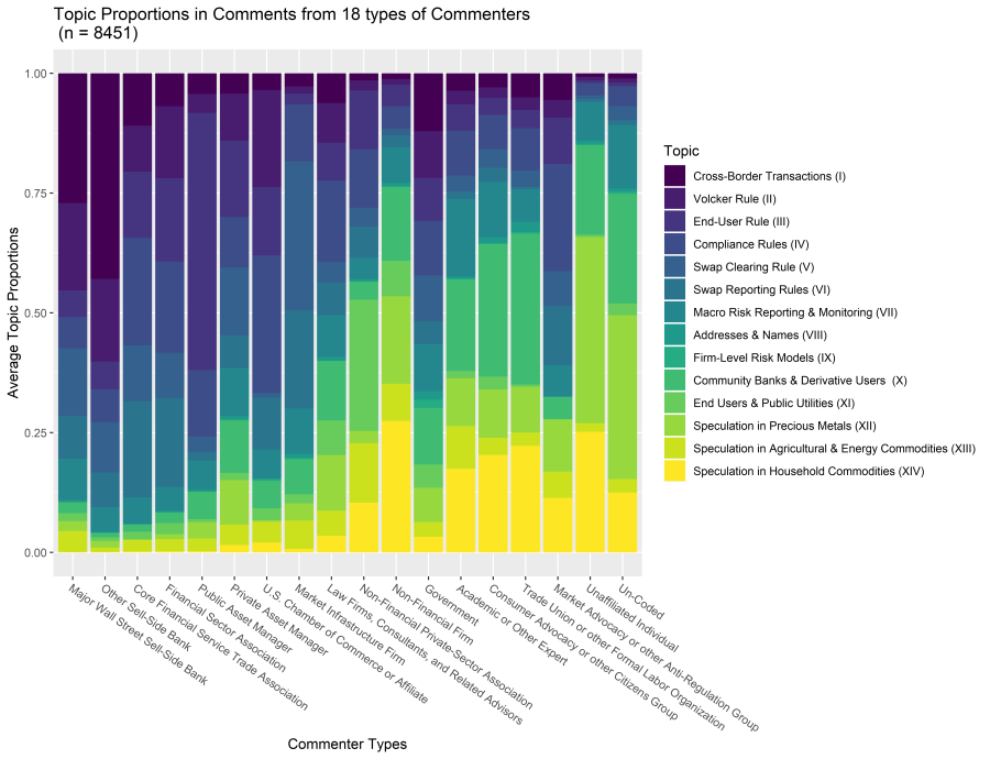
2.3.4 Generate a Heat-Map Table of Topic Proportions
The heat map greatly assists in noticing patterns in the propensity table.
The output is saved to a png file with a descriptive name.
2.3.4.1 Color Landscape Heatmap
## make a nice heatmap of the proportions
# this is the table thing where cells are colored white low to red high.  It is useful for noticing patterns in topics

filename = paste(iterations," iterations/","Topic_Proportions_by_Commenter_Type_heatmap_",n.topics,"_topics_","landscape_",format(Sys.time(), "%Y-%m-%d_%H.%M.%S"),".png", sep="")

# Note that default resolution (res) in ggplot is 72 dpi. So, to get a perfect reproduction of debug dimensions but at arbitrarily higher resolution, we simply divide the px size by 72, change unit to in, and set the res.
png(filename = paste("",filename,sep=""), width = 1100/72, height = 578/72, units = "in", res = 600)

heatmapLandscape <- ggplot(tempPlot, aes(Classifications.with.Multivalue, topic)) +
  geom_tile(aes(fill = Proportions), color= "white") +
  theme_bw() +
  xlab("") + #blank to avoid conflict with labels below
  ylab("") + #blank to avoid conflict with labels below
  scale_fill_gradient2(low = "#1A3C71", #cal Poster Template Blue
                       mid = "white",
                       high = "#FFB800", #Cal Poster Template Gold
                       midpoint = mean(tempPlot$Proportions)) + # set the scale mean at the data mean
  theme(axis.text.x=element_text(angle=35,hjust=1,vjust=1)) +
  geom_text(aes(label = round(Proportions, 4)), size=4) +
  scale_y_discrete(limits = rev(levels(tempPlot$topic)))

heatmapLandscape

dev.off()
## png
## 2## Attached image to output as well in order to enrich Rmd online appendix
include_graphics(filename)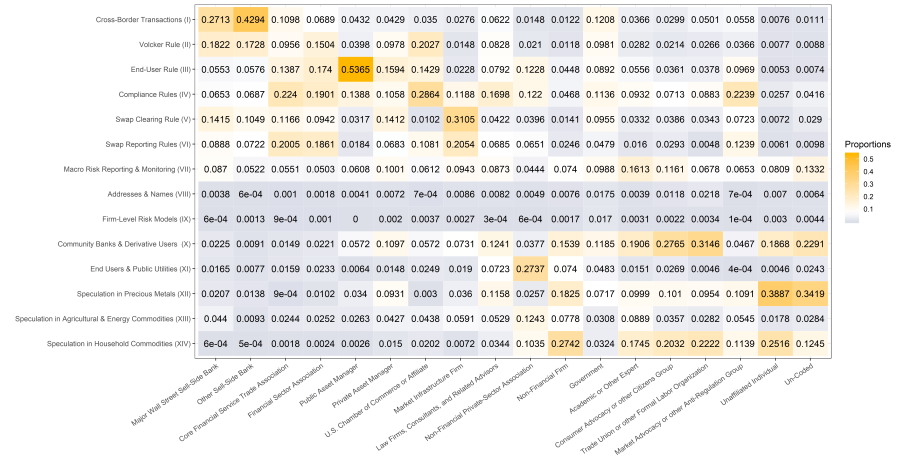
2.3.4.2 Color Portrait Heatmap
## make a nice heatmap of the proportions
# this is the table thing where cells are colored white low to red high.  It is useful for noticing patterns in topics

filename = paste(iterations," iterations/","Topic_Proportions_by_Commenter_Type_heatmap_",n.topics,"_topics_","portrait_",format(Sys.time(), "%Y-%m-%d_%H.%M.%S"),".png", sep="")

# Note that default resolution (res) in ggplot is 72 dpi. So, to get a perfect reproduction of debug dimensions but at arbitrarily higher resolution, we simply divide the px size by 72, change unit to in, and set the res.
png(filename = paste("",filename,sep=""), width = 1000/72, height = 578/72, units = "in", res = 600)

heatmapPortrait <- ggplot(tempPlot, aes(Classifications.with.Multivalue, topic)) +
  geom_tile(aes(fill = Proportions), color= "white") +
  theme_bw() +
  xlab("") + #blank to avoid conflict with labels below
  ylab("") + #blank to avoid conflict with labels below
  scale_fill_gradient2(low = "#1A3C71", #cal Poster Template Blue
                       mid = "white",
                       high = "#FFB800", #Cal Poster Template Gold
                       midpoint = mean(tempPlot$Proportions) # set the scale mean at the data mean
                       ) +
  theme(axis.text.x=element_text(angle=35,hjust=1,vjust=1)) +
  geom_text(aes(label = round(Proportions, 4)), size=4) +
  scale_x_discrete(limits = rev(levels(tempPlot$Classifications.with.Multivalue))) +
  coord_flip()

heatmapPortrait

dev.off()
## png
## 2## Attached image to output as well in order to enrich Rmd online appendix
include_graphics(filename)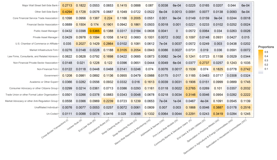
2.4 Sample of Representative Comment Letters from Each Topic
To supplement and verify the computational topic model’s analysis of the comment corpus, this section selects comment letters which exemplify each of the topics. Several strategies of selecting “exemplary” comments are used in the sections below.
2.4.1 Select ALL Comment Letters which are {1,2} standard deviations above the mean topic proportions
This first section selects all comment letters which are at least N standard deviations above the mean topic proportions for each topic, where is N is {1,2}. These letters should contain the strongest representation of each topic to display what that topic looks like in its pureset form.
It seems like 1 and 2 deviations give a very large number of letters (hundreds). numDeviationsAbove = 5 seems to give about 100 which is still more than we are interested in. This is based on testing with the topic swap.foreign.regul and may be a different pattern for other topics. 5 is too high for some topics though since there are some topics which do not have a comment which is that far away from mean. 2 creates too big a set with duplicates.
With this in mind, I will be deprecating this approach and shifting to the “top 5 approach” in 2.4.2.
# set the number of standard deviations above mean which will be used
numDeviationsAbove = 2

# create output dataframe
sampleCommentLetters_DeviationsAbove <- documents.withTopicsAndMultivalues[FALSE,]


# get the list of topic variables names in substantive (and thus df consistent) order from section 2.2
topicNamesOrdered <- names(doc.topics.IDnumbered)[2:length(names(doc.topics.IDnumbered))] #we drop the first variable name because it is ControlNumberID which is not relevant here

#### Start Loop Here ####
for (currentTopicName in topicNamesOrdered){ # wrap the entire algorithm in a loop to execute through all of the the topics

#get the mean and standard deviation
meanOfTopicProportion <- mean(documents.withTopicsAndMultivalues[,currentTopicName])
stdevOfTopicProportion <- sd(documents.withTopicsAndMultivalues[,currentTopicName])

# Start by creating a new dataframe which selects out docs which are numDeivationsAbove above the mean
currentTopicSample <- documents.withTopicsAndMultivalues[documents.withTopicsAndMultivalues[,currentTopicName]>=(meanOfTopicProportion+(numDeviationsAbove*stdevOfTopicProportion)),]

# Add a variable to CurrentTopicSample to capture which topic the comment is selected for
currentTopicSample$relevantTopic <- currentTopicName

## Add these selected documents to the sampling dataframe
sampleCommentLetters_DeviationsAbove <-
  rbind(sampleCommentLetters_DeviationsAbove, currentTopicSample)

#
}
## END OF LOOP ###

## Check if Duplicates have been added
length(unique(sampleCommentLetters_DeviationsAbove$ControlNumberID))


## Write the table to a | delimited file for easy copy into excel
filename = paste(iterations," iterations/","Sample_Comment_Letters_",numDeviationsAbove,"_Deviations_Above_Mean_",n.topics,"_topics_",format(Sys.time(), "%Y-%m-%d_%H.%M.%S"),".txt", sep="")

write.table(typologyTopicProportions, row.names=FALSE, col.names=TRUE, file = filename, sep = "|")
2.4.2 Select Top XX highest topic proportion Comment Letters
As compared to 2.4.1, this is an even more extreme selection criteria although it may be susceptible to highly clusters topic proportions since it does not verify how extreme.
This was the analysis that ultimately was most useful for understanding what letters were in topics. However, 2.4.1 and 2.4.3 are retained in specification and partial implementation for posterity in case a future analyst wishes to explore alternative meanings of “typical” or “representative” when evaluating topics.
# set the number of comments to be selected from the top of the distribution
topNumSelected = 30

#create working copy of documents.withTopics dropping unnneded metadata
#   Note: we do NOT need to use multivalues for this strict "top ranking" selection criteria since we are not selecting in comparison to the entire corpus as we would be with the stdev or porportion models.
names(documents.withTopics)
## [1] "ControlNumberID"
## [2] "SubmitDate"
## [3] "UniqueName"
## [4] "FirstName"
## [5] "LastName"
## [6] "Organization"
## [7] "Title"
## [8] "In.NZ.and.LE.memos"
## [9] "Rule.Super.set..from.Memo.Title."
## [10] "Final.Classification"
## [11] "Final.Classification.Multivalue.2"
## [12] "Final.Classification.Multivalue.3"
## [13] "Final.Classification.Multivalue.4"
## [14] "Final.Classification.Multivalue.5"
## [15] "VA.KSC.Classification"
## [16] "VA.KSC.Multivalue.2"
## [17] "VA.KSC.Multivalue.3"
## [18] "VA.KSC.Multivalue.4"
## [19] "VA.KSC.Multivalue.5"
## [20] "VA.KSC.Non.US...Non.US.or.Blank."
## [21] "LE.Non.US...Non.US.or.Blank."
## [22] "LE.Classification"
## [23] "CommentText"
## [24] "ExtractedText"
## [25] "UnifiedText"
## [26] "PreppedText"
## [27] "swap.dealer.foreign"
## [28] "fund.bank.entiti"
## [29] "swap.requir.risk"
## [30] "commiss.requir.complianc"
## [31] "clear.requir.custom"
## [32] "swap.report.requir"
## [33] "risk.liquid.price"
## [34] "ca.ny.fl"
## [35] "cio.occ.jpmorgan"
## [36] "bank.doddfrank.state"
## [37] "swap.energi.commiss"
## [38] "silver.limit.contract"
## [39] "posit.limit.commod"
## [40] "specul.commod.price"
## [41] "Classifications.with.Multivalue"documents.ToSample <- documents.withTopics[,c(
1:6,
25,
27:40,
10
)]
# create output dataframe, on re-runs, note that this also blanks out previous sample data which is desireable behavior to prevent accidents.
sampleCommentLetters_topNumber <- documents.withTopics[FALSE,]
# get the list of topic variables names in substantive (and thus df consistent) order from section 2.2
topicNamesOrdered <- names(doc.topics.IDnumbered)[2:length(names(doc.topics.IDnumbered))] #we drop the first variable name because it is ControlNumberID which is not relevant here
#### Start Loop Here ####
for (currentTopicName in topicNamesOrdered){ # wrap the entire algorithm in a loop to execute through all of the the topics
#create temp working dataframe from topics without multivalues
tempCommentsByTopics <- documents.ToSample[order(-documents.ToSample[,currentTopicName]),]
# Create a new dataframe which selects out docs which are in the topNumSelected
currentTopicSample <- tempCommentsByTopics[1:topNumSelected,]
# Add a variable to CurrentTopicSample to capture which topic the comment is selected for
currentTopicSample$relevantTopic <- currentTopicName
## Add these selected documents to the sampling dataframe
sampleCommentLetters_topNumber <-
rbind(sampleCommentLetters_topNumber, currentTopicSample)
#
}
## END OF LOOP ###
## Are there duplicate Comment Letters? (False means no because we are comparing the number of unique comment IDs to the total number of comments)
length(unique(sampleCommentLetters_topNumber$ControlNumberID)) != nrow(sampleCommentLetters_topNumber)## [1] FALSE## Change relevantTopic to factor and rename levels to descriptive names
sampleCommentLetters_topNumber$relevantTopic <- factor(sampleCommentLetters_topNumber$relevantTopic)
sampleCommentLetters_topNumber$relevantTopic <- mapvalues(sampleCommentLetters_topNumber$relevantTopic,
from = topicNamesOrdered, #
to = c(
"Cross-Border Transactions (I)",
"Volcker Rule (II)",
"End-User Rule (III)",
"Compliance Rules (IV)",
"Swap Clearing Rule (V)",
"Swap Reporting Rules (VI)",
"Macro Risk Reporting & Monitoring (VII)",
"Addresses & Names (VIII)",
"Firm-Level Risk Models (IX)",
"Community Banks & Derivative Users (X)",
"End Users & Public Utilities (XI)",
"Speculation in Precious Metals (XII)",
"Speculation in Agricultural & Energy Commodities (XIII)",
"Speculation in Household Commodities (XIV)"
))
## Put the relevant topic variables at the front and relevant comment letter text at the end
sampleCommentLetters_topNumber <- sampleCommentLetters_topNumber[,c(23,22,1:6,8:21,7)]
## Create a directory to hold this large number of letters
letterDirectory <- paste(wd,"/",iterations," iterations/Letters/", sep="")
dir.create(letterDirectory)## Warning in dir.create(letterDirectory): 'D:\Dropbox\The Limits of
## Interest\12000 iterations\Letters' already exists## Write each selected letter to a SEPERATE file with it's metadata
for ( commentNum in 1:nrow(sampleCommentLetters_topNumber)){
currentLetter <- sampleCommentLetters_topNumber[commentNum,]
if (commentNum%%topNumSelected == 0)
{
currentRank <- topNumSelected
} else {
currentRank <- commentNum%%topNumSelected
}
filename = paste(letterDirectory, "/",
currentLetter[1,1],"_Letter_#",
currentRank,
"_",
format(Sys.time(), "%Y-%m-%d_%H.%M.%S"),
".txt",
sep="")
for ( varNum in 1:ncol(currentLetter) ){
write(c(paste(as.character(colnames(currentLetter)[varNum]), ## This is the variable name
as.character(currentLetter[1,varNum]), ## This is the variable value
sep = " : ")
),
file = filename,
append = TRUE
)
}
}
#NOTE: Due to the excel cell character limit, example letters need to be outputted as individual files
# and then copied manually into word files for full text. But, a tabular comparison file is useful
#
## Write the table to a | delimited file for easy copy into excel
filename = paste(letterDirectory,"/","Sample_Comment_Letters_TRUNCATED_Top_",topNumSelected,"_by_Proportions_",n.topics,"_topics_",format(Sys.time(), "%Y-%m-%d_%H.%M.%S"),".txt", sep="")
write.table(sampleCommentLetters_topNumber, row.names=FALSE, col.names=TRUE, file = filename, sep = "|")2.4.3 Select Median 5 Comment letters closest to the median Topic Proportion
This selection emphasizes the “typical” usage of the topic in the corpus but will likely, for that reason, be more difficult to isolate the essence of the specific topic. However, it may be useful should there be concerns about misrepresentativeness of extreme proportion selections in 2.4.1 and 2.4.2
3. Who Commented on the 10 most commented rules in the Coded (8k) dataset
Now we want to see who was commenting on the 10 most commented on rules. This data primarily discussed in Supporting Information B and E.
3.1 The top 10 Rules by number of comments
First, we need that top 10 list. Note: This will be based on the coded comments only, which is the set of 8568 comments not the set of 37,232 comments.
# reset the working dataframe to the backup to ensure clean data for every step
documents.withTopicsAndMultivalues <- documents.withTopicsAndMultivaluesBKUP_2.2

# get the unique list of rules with counts of relevant comments
cftc.Comments.coded.counts <- as.data.frame(table(documents.withTopicsAndMultivalues$UniqueName))

colnames(cftc.Comments.coded.counts)[1]<- "UniqueName"
colnames(cftc.Comments.coded.counts)[2]<- "Comments"

## Sort in decending order of frequency to see top values
cftc.Comments.coded.counts <- cftc.Comments.coded.counts[order(cftc.Comments.coded.counts$Comments, decreasing = TRUE),]

# examine the top 15 rules to get a sense for patterns
head(cftc.Comments.coded.counts, 15)
## UniqueName Comments
## 67 76 FR 4752 3335
## 38 75 FR 80747 659
## 1 75 FR 3281 432
## 101 77 FR 8332 377
## 35 75 FR 80174 261
## 6 75 FR 63732 185
## 93 77 FR 41213 168
## 107 78 FR 75680 153
## 42 76 FR 1214 129
## 82 77 FR 15460 113
## 2 75 FR 51429 106
## 27 75 FR 76139 102
## 37 75 FR 80638 92
## 56 76 FR 29818 92
## 52 76 FR 23732 82## get the top 10
top.commented.rules <- head(cftc.Comments.coded.counts,n = 10)
#simple print
top.commented.rules## UniqueName Comments
## 67 76 FR 4752 3335
## 38 75 FR 80747 659
## 1 75 FR 3281 432
## 101 77 FR 8332 377
## 35 75 FR 80174 261
## 6 75 FR 63732 185
## 93 77 FR 41213 168
## 107 78 FR 75680 153
## 42 76 FR 1214 129
## 82 77 FR 15460 113# write all rule counts to csv for simple excel manipulation/copy paste
write.csv(cftc.Comments.coded.counts, file=paste(iterations," iterations/","Comments_Top10Rules_n",sum(top.commented.rules$NumberOfComments),format(Sys.time(), "%Y-%m-%d_%H.%M.%S"),".csv", sep=""), row.names = FALSE)
# latex table for publishing etc.
print(xtable(top.commented.rules), include.rownames = FALSE)## % latex table generated in R 3.6.1 by xtable 1.8-4 package
## % Sun Dec 01 12:44:09 2019
## \begin{table}[ht]
## \centering
## \begin{tabular}{lr}
## \hline
## UniqueName & Comments \\
## \hline
## 76 FR 4752 & 3335 \\
## 75 FR 80747 & 659 \\
## 75 FR 3281 & 432 \\
## 77 FR 8332 & 377 \\
## 75 FR 80174 & 261 \\
## 75 FR 63732 & 185 \\
## 77 FR 41213 & 168 \\
## 78 FR 75680 & 153 \\
## 76 FR 1214 & 129 \\
## 77 FR 15460 & 113 \\
## \hline
## \end{tabular}
## \end{table}3.2 Getting the comments from the coded dataset
# reset the working dataframe to the backup to ensure clean data for every step
documents.withTopicsAndMultivalues <- documents.withTopicsAndMultivaluesBKUP_2.2

# create the top 10 rule comment dataset
cftc.Comments.coded.top10 <- subset(documents.withTopicsAndMultivalues, UniqueName %in% top.commented.rules$UniqueName)

# create the inverse as well
cftc.Comments.coded.11toEnd <- subset(documents.withTopicsAndMultivalues, !(UniqueName %in% top.commented.rules$UniqueName))


# check that the number of comments pulled is the sum total of the number in the top 10 list
nrow(cftc.Comments.coded.top10)
## [1] 5812sum(top.commented.rules$NumberOfComments)## [1] 03.3 Stacked Bar Charts of Commenter type
Now that we have the comments pulled out, we’ll use this dataset to generate some stacked bar charts.
3.3.1 Top 10 Rules Combined
First, the pool of comments for all 10 rules combined.
all.comments = x=factor("All Rules") ##dummy factor to produce a stacked bar chart with only one bar.

chartTitle = "Most Frequently Commented Ten CFTC Proposed Rules:\nComments by Type of Organization"
filename=paste(iterations," iterations/","Comments_by_OrgType_Top10Rules_n",nrow(cftc.Comments.coded.top10),"_",format(Sys.time(), "%Y-%m-%d_%H.%M.%S"),".png", sep="")

png(filename = paste(filename,sep=""), width = 753/72, height = 578/72, units = "in", res=600)

topTenCombinedBar <- ggplot(cftc.Comments.coded.top10,
       aes(all.comments,
           fill=Classifications.with.Multivalue,
           order=-as.numeric(Classifications.with.Multivalue))) +
  geom_bar() +
  scale_fill_viridis(name="Commenter Type", discrete = TRUE,
                      labels=paste(levels(cftc.Comments.coded.top10$Classifications.with.Multivalue),
                                   " (",
                                   table(cftc.Comments.coded.top10$Classifications.with.Multivalue),
                                   ")",sep=""))  +
  xlab("") +
  ylab("Number of Comments") +
  labs(title=paste(chartTitle,"\n (n = ",nrow(cftc.Comments.coded.top10),")", sep=""))

topTenCombinedBar

dev.off()
## png
## 2## Attach image to output as well in order to enrich Rmd online appendix
include_graphics(filename)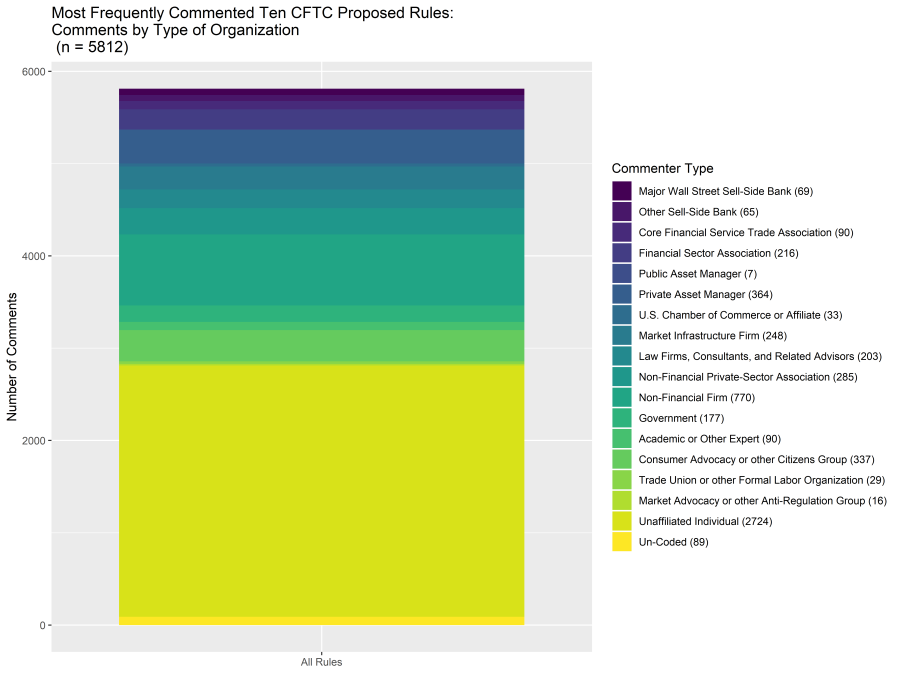
3.3.2 11 to N Rules Combined for Comparison
For comparison, let’s also look at the inverse: the 11th through end rules
all.comments = x=factor("All Rules") ##dummy factor to produce a stacked bar chart with only one bar.

chartTitle = "Less Frequently Commented (11 to 114) CFTC Proposed Rules:\nComments by Type of Organization"
filename=paste(iterations," iterations/","Comments_by_OrgType_11toEnd_n",nrow(cftc.Comments.coded.11toEnd),"_",format(Sys.time(), "%Y-%m-%d_%H.%M.%S"),".png", sep="")

png(filename = paste(filename,sep=""), width = 753/72, height = 578/72, units = "in", res=600)

elevenToEndCombinedBar <- ggplot(cftc.Comments.coded.11toEnd,
                                 aes(all.comments,
                                     fill=Classifications.with.Multivalue,
                                     order=-as.numeric(Classifications.with.Multivalue))) +
  geom_bar() +
  scale_fill_viridis(name="Commenter Type", discrete = TRUE,
                      labels=paste(levels(cftc.Comments.coded.top10$Classifications.with.Multivalue),
                                   " (",
                                   table(cftc.Comments.coded.top10$Classifications.with.Multivalue),
                                   ")",sep="")) +
  xlab("") + ylab("Number of Comments") +
  labs(title=paste(chartTitle,"\n (n = ",nrow(cftc.Comments.coded.11toEnd),")", sep=""))

elevenToEndCombinedBar

dev.off()
## png
## 2## Attach image to output as well in order to enrich Rmd online appendix
include_graphics(filename)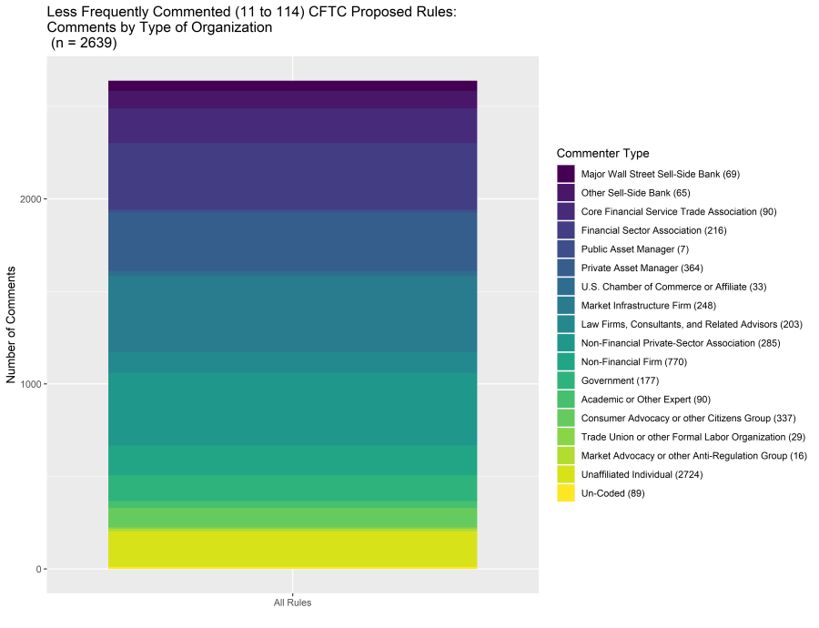
3.4 Top 10 Commented Rules split out by Rule
Then, we also want to see each of the 10 rules split out.
3.4.1 Top 1 to 10 Rules Split Out
chartTitle = "Most Frequently Commented Ten CFTC Proposed Rules:\nComments by Type of Organization per Rule"
filename=paste(iterations," iterations/","Comments_by_OrgType_Top10Rules_splitout_n",nrow(cftc.Comments.coded.top10),"_",format(Sys.time(), "%Y-%m-%d_%H.%M.%S"),".png", sep="")

# NOTE: in order to get the rules sorted by descending order of volume of comments, we on-the-fly cast  UniqueName into a factor with levels from the top.commented.rules table created earlier which has the names of the rules sorted in descending order of comment volume.  This happens in the aes argument of the ggplot function

png(filename = paste(filename,sep=""), width = 753/72, height = 578/72, units = "in", res=600)

topTenSplitBar <- ggplot(cftc.Comments.coded.top10,
                         aes(factor(UniqueName,levels = top.commented.rules$UniqueName),
                             fill=Classifications.with.Multivalue,
                             order=-as.numeric(Classifications.with.Multivalue))) +
  geom_bar()+
  theme(axis.text.x=element_text(angle=20,
                                 hjust=.75,
                                 vjust=1)) +
  scale_fill_viridis(name="Commenter Type", discrete=TRUE) +
  xlab("Top 10 Commented Rules") +
  ylab("Number of Comments") +
  labs(title=paste(chartTitle,"\n (n = ",nrow(cftc.Comments.coded.top10),")", sep=""))

topTenSplitBar

dev.off()
## png
## 2## Attach image to output as well in order to enrich Rmd online appendix
include_graphics(filename)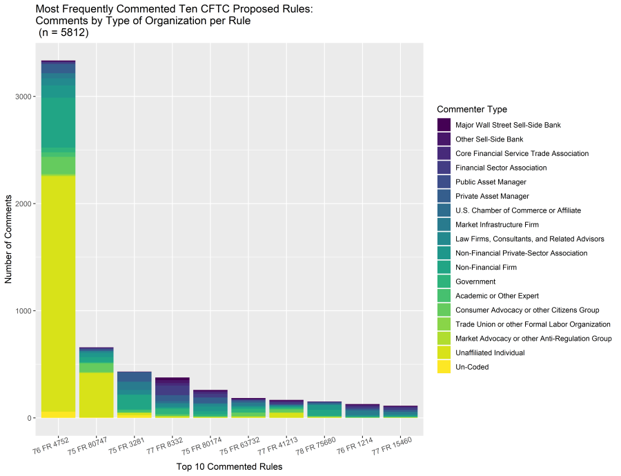
### This lets you try it facetted instead, but the results are poor.  Maintained for archival purposes
# png(filename = "../Results/Comments_top10_by_Rule_facets.png", width = 753, height = 578, units = "px")
# ggplot(cftc.Comments.coded.top10, aes(all.comments, fill=Classifications.with.Multivalue, order=-as.numeric(Classifications.with.Multivalue))) + geom_bar() + scale_fill_discrete()  + xlab("") + ylab("Number of Comments") +labs(title=paste("All Comments on the Top 10 Commented CFTC Proposed Rules to Implement the Dodd-Frank Act\n (n =",nrow(cftc.Comments.coded.top10),")")) + facet_wrap(~UniqueName)
# dev.off()
3.4.2 Top 2 to 10 Rules (For easier comparison)
Now, let’s drop the first rule (76 FR 4752) since it is so many more comments than the other rules Then, we also want to see each of the 10 rules split out.
# create the top 2to10 rule comment dataset
cftc.Comments.coded.top2thru10 <- subset(cftc.Comments.coded.top10, UniqueName !="76 FR 4752")


chartTitle = "(2nd to 10th) Most Frequently Commented CFTC Proposed Rules:\nComments by Type of Organization per Rule"
filename=paste(iterations," iterations/","Comments_by_OrgType_Top2thru10Rules_splitout_n",nrow(cftc.Comments.coded.top2thru10),"_",format(Sys.time(), "%Y-%m-%d_%H.%M.%S"),".png", sep="")

# NOTE: in order to get the rules sorted by descending order of volume of comments, we on-the-fly cast  UniqueName into a factor with levels from the top.commented.rules table created earlier which has the names of the rules sorted in descending order of comment volume.  This happens in the aes argument of the ggplot function

png(filename = paste(filename,sep=""), width = 753/72, height = 578/72, units = "in", res=600)

twoToTenSplitBar <- ggplot(cftc.Comments.coded.top2thru10,
                           aes(factor(UniqueName,
                                      levels = top.commented.rules$UniqueName),
                               fill=Classifications.with.Multivalue,
                               order=-as.numeric(Classifications.with.Multivalue))) +
  geom_bar()+
  theme(axis.text.x=element_text(angle=20,
                                 hjust=.75,
                                 vjust=1)) +
  scale_fill_viridis(name="Commenter Type", discrete=TRUE) +
  xlab("Top 2 to 10 Commented Rules") +
  ylab("Number of Comments") +
  labs(title=paste(chartTitle,"\n (n = ",nrow(cftc.Comments.coded.top2thru10),")", sep=""))

twoToTenSplitBar

dev.off()
## png
## 2## Attach image to output as well in order to enrich Rmd online appendix
include_graphics(filename)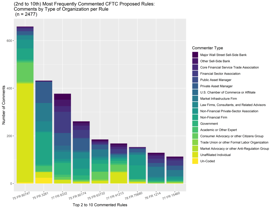
3.5 Create a Table of the number of comments by type for each of the top 10 rules
because we cannot include the totals in a clear way in the legend of the 10-bar stacked chart, we need a quick cross-tabs table to give us the totals for each rule. We’ll use the table function to accomplish this.
cftc.Comments.coded.top10.counts <- table(cftc.Comments.coded.top10$Classifications.with.Multivalue,factor(cftc.Comments.coded.top10$UniqueName,levels = top.commented.rules$UniqueName))

#Quick print to console, but this is not useful for copy/paste because window is too narrow
cftc.Comments.coded.top10.counts
##
## 76 FR 4752 75 FR 80747
## Major Wall Street Sell-Side Bank 7 2
## Other Sell-Side Bank 4 1
## Core Financial Service Trade Association 4 5
## Financial Sector Association 15 11
## Public Asset Manager 2 1
## Private Asset Manager 86 14
## U.S. Chamber of Commerce or Affiliate 2 2
## Market Infrastructure Firm 46 2
## Law Firms, Consultants, and Related Advisors 66 17
## Non-Financial Private-Sector Association 115 37
## Non-Financial Firm 465 47
## Government 45 6
## Academic or Other Expert 42 6
## Consumer Advocacy or other Citizens Group 160 81
## Trade Union or other Formal Labor Organization 13 6
## Market Advocacy or other Anti-Regulation Group 8 1
## Unaffiliated Individual 2197 415
## Un-Coded 58 5
##
## 75 FR 3281 77 FR 8332
## Major Wall Street Sell-Side Bank 3 25
## Other Sell-Side Bank 0 27
## Core Financial Service Trade Association 1 24
## Financial Sector Association 0 89
## Public Asset Manager 0 0
## Private Asset Manager 90 53
## U.S. Chamber of Commerce or Affiliate 0 18
## Market Infrastructure Firm 77 8
## Law Firms, Consultants, and Related Advisors 42 30
## Non-Financial Private-Sector Association 4 10
## Non-Financial Firm 136 7
## Government 6 49
## Academic or Other Expert 21 10
## Consumer Advocacy or other Citizens Group 4 11
## Trade Union or other Formal Labor Organization 0 0
## Market Advocacy or other Anti-Regulation Group 0 1
## Unaffiliated Individual 24 15
## Un-Coded 24 0
##
## 75 FR 80174 75 FR 63732
## Major Wall Street Sell-Side Bank 7 6
## Other Sell-Side Bank 11 4
## Core Financial Service Trade Association 18 7
## Financial Sector Association 33 5
## Public Asset Manager 3 1
## Private Asset Manager 50 19
## U.S. Chamber of Commerce or Affiliate 6 0
## Market Infrastructure Firm 3 30
## Law Firms, Consultants, and Related Advisors 25 7
## Non-Financial Private-Sector Association 43 8
## Non-Financial Firm 28 15
## Government 17 33
## Academic or Other Expert 3 1
## Consumer Advocacy or other Citizens Group 5 32
## Trade Union or other Formal Labor Organization 1 5
## Market Advocacy or other Anti-Regulation Group 1 1
## Unaffiliated Individual 7 11
## Un-Coded 0 0
##
## 77 FR 41213 78 FR 75680
## Major Wall Street Sell-Side Bank 6 2
## Other Sell-Side Bank 8 0
## Core Financial Service Trade Association 9 2
## Financial Sector Association 19 4
## Public Asset Manager 0 0
## Private Asset Manager 5 14
## U.S. Chamber of Commerce or Affiliate 1 1
## Market Infrastructure Firm 8 8
## Law Firms, Consultants, and Related Advisors 4 2
## Non-Financial Private-Sector Association 5 44
## Non-Financial Firm 8 57
## Government 11 2
## Academic or Other Expert 6 1
## Consumer Advocacy or other Citizens Group 26 8
## Trade Union or other Formal Labor Organization 4 0
## Market Advocacy or other Anti-Regulation Group 1 1
## Unaffiliated Individual 46 6
## Un-Coded 1 1
##
## 76 FR 1214 77 FR 15460
## Major Wall Street Sell-Side Bank 6 5
## Other Sell-Side Bank 6 4
## Core Financial Service Trade Association 13 7
## Financial Sector Association 18 22
## Public Asset Manager 0 0
## Private Asset Manager 15 18
## U.S. Chamber of Commerce or Affiliate 2 1
## Market Infrastructure Firm 41 25
## Law Firms, Consultants, and Related Advisors 6 4
## Non-Financial Private-Sector Association 9 10
## Non-Financial Firm 2 5
## Government 5 3
## Academic or Other Expert 0 0
## Consumer Advocacy or other Citizens Group 5 5
## Trade Union or other Formal Labor Organization 0 0
## Market Advocacy or other Anti-Regulation Group 0 2
## Unaffiliated Individual 1 2
## Un-Coded 0 0#write to CSV for simple data export to excel or word
write.csv(cftc.Comments.coded.top10.counts,
file=paste(iterations," iterations/", "Comments_by_OrgType_Top10Rules_splitoutTable_n",nrow(cftc.Comments.coded.top10),".csv", sep=""))
# latex type setting
xtable(cftc.Comments.coded.top10.counts)## % latex table generated in R 3.6.1 by xtable 1.8-4 package
## % Sun Dec 01 12:44:16 2019
## \begin{table}[ht]
## \centering
## \begin{tabular}{rrrrrrrrrrr}
## \hline
## & 76 FR 4752 & 75 FR 80747 & 75 FR 3281 & 77 FR 8332 & 75 FR 80174 & 75 FR 63732 & 77 FR 41213 & 78 FR 75680 & 76 FR 1214 & 77 FR 15460 \\
## \hline
## Major Wall Street Sell-Side Bank & 7 & 2 & 3 & 25 & 7 & 6 & 6 & 2 & 6 & 5 \\
## Other Sell-Side Bank & 4 & 1 & 0 & 27 & 11 & 4 & 8 & 0 & 6 & 4 \\
## Core Financial Service Trade Association & 4 & 5 & 1 & 24 & 18 & 7 & 9 & 2 & 13 & 7 \\
## Financial Sector Association & 15 & 11 & 0 & 89 & 33 & 5 & 19 & 4 & 18 & 22 \\
## Public Asset Manager & 2 & 1 & 0 & 0 & 3 & 1 & 0 & 0 & 0 & 0 \\
## Private Asset Manager & 86 & 14 & 90 & 53 & 50 & 19 & 5 & 14 & 15 & 18 \\
## U.S. Chamber of Commerce or Affiliate & 2 & 2 & 0 & 18 & 6 & 0 & 1 & 1 & 2 & 1 \\
## Market Infrastructure Firm & 46 & 2 & 77 & 8 & 3 & 30 & 8 & 8 & 41 & 25 \\
## Law Firms, Consultants, and Related Advisors & 66 & 17 & 42 & 30 & 25 & 7 & 4 & 2 & 6 & 4 \\
## Non-Financial Private-Sector Association & 115 & 37 & 4 & 10 & 43 & 8 & 5 & 44 & 9 & 10 \\
## Non-Financial Firm & 465 & 47 & 136 & 7 & 28 & 15 & 8 & 57 & 2 & 5 \\
## Government & 45 & 6 & 6 & 49 & 17 & 33 & 11 & 2 & 5 & 3 \\
## Academic or Other Expert & 42 & 6 & 21 & 10 & 3 & 1 & 6 & 1 & 0 & 0 \\
## Consumer Advocacy or other Citizens Group & 160 & 81 & 4 & 11 & 5 & 32 & 26 & 8 & 5 & 5 \\
## Trade Union or other Formal Labor Organization & 13 & 6 & 0 & 0 & 1 & 5 & 4 & 0 & 0 & 0 \\
## Market Advocacy or other Anti-Regulation Group & 8 & 1 & 0 & 1 & 1 & 1 & 1 & 1 & 0 & 2 \\
## Unaffiliated Individual & 2197 & 415 & 24 & 15 & 7 & 11 & 46 & 6 & 1 & 2 \\
## Un-Coded & 58 & 5 & 24 & 0 & 0 & 0 & 1 & 1 & 0 & 0 \\
## \hline
## \end{tabular}
## \end{table}4. Deprecated Additional Analyses
In our initial exploration of the topic models and topic proportions, these analyses were helpful to characterize the data. They are not used in the paper as they ultimately did not provide the insights which answered our research questions. They are retained here for future analysts looking to explore and characterize topic model data based on our approach.
4.1 Easily adjustable two-type comparison
Based on the 17 part proportions in 2.3, this section allows us to easily explore different commenter type combinations. It works by setting two types at the begining of the code block. To set the types, you must copy the exact name from the list below into the typeA and typeB variables.
“Major Wall Street Sell-Side Bank”, “Core Financial Service Trade Association”, “Other Sell-Side Bank”, “Public Asset Manager”, “Private Asset Manager”, “U.S. Chamber of Commerce or Affiliate”, “Market Infrastructure Firm”, “Law Firms, Consultants, and Related Advisors”, “Non-Financial Firm”, “Private-Sector Association”, “Government”, “Academic or Other Expert”, “Consumer Advocacy or other Citizens Group”, “Trade Union or other Formal Labor Organization”, “Market Advocacy or other Anti-Regulation Group”, “Unaffiliated Individual”, “Un-Coded” <———————————————————-
# reset the working dataframe to the backup to ensure clean data for every step
documents.withTopicsAndMultivalues <- documents.withTopicsAndMultivaluesBKUP_2.2

## Set the commenter types you want to compare below
groupTypes = c(
  "industryGroup"
 ,"nonIndustryGroup"
  )

# average all the documents down to the 17 part typology in Classifications.with.Multivalue

typologyTopicProportions <- ddply(
                        documents.withTopicsAndMultivalues[2:length(names(documents.withTopicsAndMultivalues))] ### omit ID
                        ,"Classifications.with.Multivalue"
                        ,numcolwise(mean))

# report the dataframe where each row is one of the commenter types from VA.KSC, and each column is a topic.  Each cell will then be the average Proportions of the commenter type to mention a particular topic.  (Does this add up to 1 always?, probably not due to averaging)

typologyTopicProportions

# now, drop all lines from typologyTopicProportions which are not typeA and typeB
typeABtopicProportions <- typologyTopicProportions[typologyTopicProportions$Classifications.with.Multivalue %in% groupTypes,]

# confirm that the correct types were retained
typeABtopicProportions


###########################
#   creation of png file  #
#   (be sure to turn on   #
#   dev.off() line after  #
#    the chart)           #
###########################
#filename = paste("Topic_Proportions_",paste(groupTypes, collapse ="&"),"_",n.topics,"_topics_",format(Sys.time(), "%Y-%m-%d_%H.%M.%S"),".png", sep="")
#png(filename = paste("",filename,sep=""), width = 753, height = 578, units = "px")


# Stacked Bar Chart of Proportions for Visual Comparison
chartTitle = paste("Topic Proportions in Comments from ",paste(groupTypes, collapse =" & ")," type Commenters", sep="")


#create a "tall" file which lists each of the variables vertically rather than a wide file where each variable is a column.
tempPlot <- melt(typeABtopicProportions, id.vars="Classifications.with.Multivalue")
colnames(tempPlot)<- c("Classifications.with.Multivalue","topic","Proportions") #make the names descriptive

ggplot(tempPlot, aes(Classifications.with.Multivalue, Proportions, fill=topic)) +geom_bar(stat = "identity") + theme(axis.text.x=element_text(angle=0,hjust=.5,vjust=1)) + xlab("Commenter Types") + ylab("Average Topic Proportions") +labs(title=paste(chartTitle,"\n (#topics = ",n.topics,")", sep=""))

###############
#dev.off()
###############

## make a nice pseudo-table of the Proportions
# this is the weird green circle table-type thing that we came up with since R doesn't do tables well.

#filename = paste("Topic_Proportions_",paste(groupTypes, collapse ="&"),"_dotsplot_",n.topics,"_topics_",format(Sys.time(), "%Y-%m-%d_%H.%M.%S"),".png", sep="")
#png(filename = paste("",filename,sep=""), width = 1000, height = 578, units = "px")

#g <- ggplot(tempPlot, aes(Classifications.with.Multivalue, topic)) + geom_point(aes(size = Proportions), color= "green") + theme_bw() + xlab("") + ylab("")
#g + scale_size_continuous(range=c(1,10)) + theme(axis.text.x=element_text(angle=35,hjust=1,vjust=1))  + geom_text(aes(label = round(Proportions, 4)), size=4)

#dev.off()
4.2 Basic Binary Industry vs. Non-Industry comparison
Following the data presentation in (Levy & Franklin 2014), we begin by presenting a comparison between two halves of the data: those commenter types who can be considered Industry and those which are non-Industry organization, academics, and private individuals.
Based on the 17 part typology Industry “Major Wall Street Sell-Side Bank”, “Core Financial Service Trade Association”, “Other Sell-Side Bank”, “Public Asset Manager”, “Private Asset Manager”, “U.S. Chamber of Commerce or Affiliate”, “Market Infrastructure Firm”, “Law Firms, Consultants, and Related Advisors”, “Non-Financial Firm”, “Financial Sector Association”, “Non-Financial Private-Sector Association”,
Non-Industry “Government”, “Academic or Other Expert”, “Consumer Advocacy or other Citizens Group”, “Trade Union or other Formal Labor Organization”, “Market Advocacy or other Anti-Regulation Group”, “Unaffiliated Individual”, “Un-Coded” <———————————————————-
# reset the working dataframe to the backup to ensure clean data for every step
documents.withTopicsAndMultivalues <- documents.withTopicsAndMultivaluesBKUP_2.2

# add in the Industry binary as a variable to our documents.withTopic dataframe

industryClassification<-c("Industry","Industry","Industry","Industry","Industry","Industry","Industry","Industry","Industry","Industry","Industry","Non-Industry","Non-Industry","Non-Industry","Non-Industry","Non-Industry","Non-Industry","")
### Last classification is blank and represents the Uncoded category.
### Omit blank line from furter analysis

indusClassificationDF <- data.frame(typology,industryClassification)

indusClassificationDF

temp <- merge(documents.withTopicsAndMultivalues, indusClassificationDF, by.x = "Classifications.with.Multivalue", by.y="typology")


# average documents to two lines and N topics columns based on the list above
industryBinaryTopicProportions <- ddply(
                        documents.withTopicsAndMultivalues[3:length(names(documents.withTopicsAndMultivalues))] ### omit ID
                        ,"industryClassification"
                        ,numcolwise(mean))


# report the dataframe where each row is one of the commenter types from VA.KSC, and each column is a topic.

industryBinaryTopicProportions

#to count the number of comments in each super type:
sum(1*(temp$industryClassification=="Industry"))
sum(1*(temp$industryClassification=="Non-Industry"))

#drop the uncoded
industryBinaryTopicProportions <- industryBinaryTopicProportions[2:nrow(industryBinaryTopicProportions),]

# report as a table where each cell is the Proportions of group [row] to mention topic [column]. Each cell will then be the average Proportions of the commenter super-type to mention a particular topic.  (Does this add up to 1 always?, probably not due to averaging, but it's pretty close)

# Stacked Bar Chart of Proportions for Visual Comparison
chartTitle = "Topic Proportions in Comments from Industry and Non-Industry"
filename = paste("Topic_Proportions_by_Industry_NonIndustry_",n.topics,"_topics_",format(Sys.time(), "%Y-%m-%d_%H.%M.%S"),".png", sep="")

tempPlot <- melt(industryBinaryTopicProportions, id.vars="industryClassification")
colnames(tempPlot)<- c("industryClassification","topic","Proportions")

png(filename = paste("",filename,sep=""), width = 753, height = 578, units = "px")

ggplot(tempPlot, aes(industryClassification, Proportions, fill=topic)) +geom_bar(stat = "identity") + theme(axis.text.x=element_text(angle=35,hjust=1,vjust=1)) + xlab("Commenter Types") + ylab("Average Topic Proportions") +labs(title=paste(chartTitle,"\n (n = ",nrow(documents.withTopicsAndMultivalues),")", sep=""))

dev.off()

# make a nice pseudo-table of the Proportions

filename = paste("Topic_Proportions_by_Industry_NonIndustry_dotsplot_",n.topics,"_topics_",format(Sys.time(), "%Y-%m-%d_%H.%M.%S"),".png", sep="")
png(filename = paste("",filename,sep=""), width = 1000, height = 578, units = "px")
g <- ggplot(tempPlot, aes(industryClassification, topic)) + geom_point(aes(size = Proportions), color= "green") + theme_bw() + xlab("") + ylab("")
g + scale_size_continuous(range=c(1,10)) + theme(axis.text.x=element_text(angle=35,hjust=1,vjust=1))  + geom_text(aes(label = round(Proportions, 4)), size=4)
dev.off()
4.3 Four part comparison of Supertypes
Based on the 17 part typology
Industry Sell-Side
“Major Wall Street Sell-Side Bank”, “Core Financial Service Trade Association”, “Other Sell-Side Bank”,
Industry Buy-Side (Derivative and Commodity Users)
“Public Asset Manager”, “Private Asset Manager”, “Non-Financial Firm”, “Financial Sector Association”, “Non-Financial Private-Sector Association”,
Industry Joint Sell-Side and Buy-Side
“U.S. Chamber of Commerce or Affiliate”, “Market Infrastructure Firm”, “Law Firms, Consultants, and Related Advisors”,
Non-Industry Organizations and Individuals
“Government”, “Academic or Other Expert”, “Consumer Advocacy or other Citizens Group”, “Trade Union or other Formal Labor Organization”, “Market Advocacy or other Anti-Regulation Group”, “Unaffiliated Individual”,
This group is dropped as it is categorically not categorizable
“Un-Coded” <———————————————————-
# reset the working dataframe to the backup to ensure clean data for every step
documents.withTopicsAndMultivalues <- documents.withTopicsAndMultivaluesBKUP_2.2

# add in the Industry binary as a variable to our documents.withTopic dataframe

superType<-c(
   "Industry Sell-Side"
  ,"Industry Joint Sell-Side and Buy-Side"
  ,"Industry Sell-Side"
  ,"Industry Buy-Side (Derivative and Commodity Users)"
  ,"Industry Buy-Side (Derivative and Commodity Users)"
  ,"Industry Joint Sell-Side and Buy-Side"
  ,"Industry Joint Sell-Side and Buy-Side"
  ,"Industry Joint Sell-Side and Buy-Side"
  ,"Industry Buy-Side (Derivative and Commodity Users)"
  ,"Industry Buy-Side (Derivative and Commodity Users)"
  ,"Industry Buy-Side (Derivative and Commodity Users)"
  ,"Non-Industry"
  ,"Non-Industry"
  ,"Non-Industry"
  ,"Non-Industry"
  ,"Non-Industry"
  ,"Non-Industry"
  ,"")

superTypeDF <- data.frame(typology,superType)

superTypeDF

rm(temp)
temp <- merge(documents.withTopicsAndMultivalues, superTypeDF, by.x = "Classifications.with.Multivalue", by.y="typology" )


##Note: there are 96 blanks due to the "Uncoded"" classification
sum(1*(temp$superType==""))

#to count the number of comments in each super type:
sum(1*(temp$superType=="Industry Sell-Side"))
sum(1*(temp$superType=="Industry Joint Sell-Side and Buy-Side"))
sum(1*(temp$superType=="Industry Buy-Side (Derivative and Commodity Users)"))
sum(1*(temp$superType=="Non-Industry"))

# average documents to two lines and N topics columns based on the list above
superTypeTopicProportions <- ddply(
                        documents.withTopicsAndMultivalues[3:length(names(documents.withTopicsAndMultivalues))] ### omit ID
                        ,"superType"
                        ,numcolwise(mean))


# report the dataframe where each row is one of the commenter superTypes and each column is a topic.

superTypeTopicProportions

#drop the uncoded
superTypeTopicProportions <- superTypeTopicProportions[2:nrow(superTypeTopicProportions),]

# report as a table where each cell is the Proportions of group [row] to mention topic [column]. Each cell will then be the average Proportions of the commenter super-type to mention a particular topic.  (Does this add up to 1 always?, probably not due to averaging, but it's pretty close)

# Stacked Bar Chart of Proportions for Visual Comparison
chartTitle = "Topic Proportions in Comments from 4 Super Types"
filename = paste("Topic_Proportions_by_SuperType_",n.topics,"_topics_",format(Sys.time(), "%Y-%m-%d_%H.%M.%S"),".png", sep="")

tempPlot <- melt(superTypeTopicProportions, id.vars="superType")
colnames(tempPlot)<- c("superType","topic","Proportions")

png(filename = paste("",filename,sep=""), width = 753, height = 578, units = "px")

ggplot(tempPlot, aes(superType, Proportions, fill=topic)) +geom_bar(stat = "identity") + theme(axis.text.x=element_text(angle=35,hjust=1,vjust=1)) + xlab("Commenter Types") + ylab("Average Topic Proportions") +labs(title=paste(chartTitle,"\n (n = ",nrow(documents.withTopicsAndMultivalues),")", sep=""))

dev.off()

# make a nice pseudo-table of the Proportions

filename = paste("Topic_Proportions_by_SuperType_dotsplot_",n.topics,"_topics_",format(Sys.time(), "%Y-%m-%d_%H.%M.%S"),".png", sep="")
png(filename = paste("",filename,sep=""), width = 1000, height = 578, units = "px")
g <- ggplot(tempPlot, aes(superType, topic)) + geom_point(aes(size = Proportions), color= "green") + theme_bw() + xlab("") + ylab("")
g + scale_size_continuous(range=c(1,10)) + theme(axis.text.x=element_text(angle=35,hjust=1,vjust=1))  + geom_text(aes(label = round(Proportions, 4)), size=5)
dev.off()
4.4 Five part comparison of Supertypes
Based on the 17 part typology
Industry Sell-Side “Major Wall Street Sell-Side Bank”, “Core Financial Service Trade Association”, “Other Sell-Side Bank”,
** Industry Buy-Side (Derivative and Commodity Users)** “Public Asset Manager”, “Private Asset Manager”, “Non-Financial Firm”, “Financial Sector Association”, “Non-Financial Private-Sector Association”,
Industry Joint Sell-Side and Buy-Side “U.S. Chamber of Commerce or Affiliate”,
Infrastructure and Market Services “Market Infrastructure Firm”, “Law Firms, Consultants, and Related Advisors”,
Non-Industry Organizations and Individuals “Government”, “Academic or Other Expert”, “Consumer Advocacy or other Citizens Group”, “Trade Union or other Formal Labor Organization”, “Market Advocacy or other Anti-Regulation Group”, “Unaffiliated Individual”,
This group is dropped as it is categorically not categorizable “Un-Coded” <———————————————————-
# reset the working dataframe to the backup to ensure clean data for every step
documents.withTopicsAndMultivalues <- documents.withTopicsAndMultivaluesBKUP_2.2

# add in the Industry binary as a variable to our documents.withTopic dataframe

FiveType<-c(
   "Industry Sell-Side"
  ,"Industry Sell-Side"
  ,"Industry Joint Sell-Side and Buy-Side"
  ,"Industry Buy-Side (Derivative and Commodity Users)"
  ,"Industry Buy-Side (Derivative and Commodity Users)"
  ,"Industry Joint Sell-Side and Buy-Side"
  ,"Infrastructure and Market Services"
  ,"Infrastructure and Market Services"
  ,"Industry Buy-Side (Derivative and Commodity Users)"
  ,"Industry Buy-Side (Derivative and Commodity Users)"
  ,"Industry Buy-Side (Derivative and Commodity Users)"
  ,"Non-Industry"
  ,"Non-Industry"
  ,"Non-Industry"
  ,"Non-Industry"
  ,"Non-Industry"
  ,"Non-Industry"
  ,"")

FiveTypeDF <- data.frame(typology,FiveType)

FiveTypeDF

rm(temp)
temp <- merge(documents.withTopicsAndMultivalues, FiveTypeDF, by.x = "Classifications.with.Multivalue", by.y="typology" )


##Note: there are 96 blanks due to the "Uncoded"" classification
sum(1*(temp$FiveType==""))
##counts number of documents with a blank

sum(1*(temp$FiveType=="Industry Sell-Side"))
sum(1*(temp$FiveType=="Industry Joint Sell-Side and Buy-Side"))
sum(1*(temp$FiveType=="Industry Buy-Side (Derivative and Commodity Users)"))
sum(1*(temp$FiveType=="Infrastructure and Market Services"))
sum(1*(temp$FiveType=="Non-Industry"))
# average documents to two lines and N topics columns based on the list above
fiveTypeTopicProportions <- ddply(
                        documents.withTopicsAndMultivalues[3:length(names(documents.withTopicsAndMultivalues))] ### omit ID
                        ,"FiveType"
                        ,numcolwise(mean))


# report the dataframe where each row is one of the commenter superTypes and each column is a topic.

fiveTypeTopicProportions

#drop the uncoded
fiveTypeTopicProportions <- fiveTypeTopicProportions[2:nrow(fiveTypeTopicProportions),]

# report as a table where each cell is the Proportions of group [row] to mention topic [column]. Each cell will then be the average Proportions of the commenter super-type to mention a particular topic.  (Does this add up to 1 always?, probably not due to averaging, but it's pretty close)

# Stacked Bar Chart of Proportions for Visual Comparison
chartTitle = "Topic Proportions in Comments In Five Super Types"
filename = paste("Topic_Proportions_by_Five_Types_",n.topics,"_topics_",format(Sys.time(), "%Y-%m-%d_%H.%M.%S"),".png", sep="")

tempPlot <- melt(fiveTypeTopicProportions, id.vars="FiveType")
colnames(tempPlot)<- c("FiveType","topic","Proportions")

png(filename = paste("",filename,sep=""), width = 753, height = 578, units = "px")

ggplot(tempPlot, aes(FiveType, Proportions, fill=topic)) +geom_bar(stat = "identity") + theme(axis.text.x=element_text(angle=35,hjust=1,vjust=1)) + xlab("Commenter Types") + ylab("Average Topic Proportions") +labs(title=paste(chartTitle,"\n (n = ",nrow(documents.withTopicsAndMultivalues),")", sep=""))

dev.off()

# make a nice pseudo-table of the Proportions
filename = paste("Topic_Proportions_by_Five_Types_dotsplot_",n.topics,"_topics_",format(Sys.time(), "%Y-%m-%d_%H.%M.%S"),".png", sep="")
png(filename = paste("",filename,sep=""), width = 1000, height = 578, units = "px")
g <- ggplot(tempPlot, aes(FiveType, topic)) + geom_point(aes(size = Proportions), color= "green") + theme_bw() + xlab("") + ylab("")
g + scale_size_continuous(range=c(1,10)) + theme(axis.text.x=element_text(angle=35,hjust=1,vjust=1))  + geom_text(aes(label = round(Proportions, 4)), size=5)
dev.off()